Statistical properties of an experimental political futures market

Abstract

A 24-hour exchange market was created on the Web to trade political futures contracts using fictitious money. In this online market, a political futures contract is a futures contract which matures on the election day with a liquidation price determined by the percentage of votes a candidate receives on the election day. Continuous double auctions were implemented as the system for order storage and price discovery. We drew market participants in the form of tournaments in which top traders won cash awards. Such a market was run, with about 400 registered traders, during the U.S. presidential election in November 2004 and Taiwan parliamentary election in December 2004. The experiments recorded transaction price, highest bid, lowest ask, and trading volume of each contract as a function of time. Despite the relatively small scale of the exchange, in terms of the number of participants and duration of the tournament, we report evidence for asymptotic power-law behaviors of the distributions of price returns, trading volumes, inter-transaction time intervals, and accumulated wealth that were found universal in real financial markets.

I Introduction

Markets are a complex system that usually consists of the following different types of participants: (i) producers who provide goods, (ii) speculators or hedgers who, with beliefs in the trends of price movements, buy low and sell high for a profit or insurance, and (iii) arbitrageurs who buy products at a low price in one market and sell them at a high price in other markets for a riskless profit. A market is liquid if sufficient numbers of the different types of players exist in symbiosis. To study the system, successive movements in observables such as price are modeled as a stochastic process due to market’s responses to the random arrivals of information. Fluctuations are predicted to be GaussianBachelier (1900) or LévyLévy (Gauthier-Villars, Paris, 1937) distributed by the central limit theorem. Distributions of large price changes, those which exceed, say, five standard deviations, however show characteristic power-law behaviorsMandelbrot (1963); Farma (1965); Dacorogna et al. (1993); Loretan and Phillips (1994); Lux (1996); Pagan (1996); Bouchaud and Potters (Alea-Saclay, Eyrolles, 1998); Arnéodo et al. (1998); Gopikrishnan et al. (1999); Plerou et al. (1999). Models to explain the power-law range from systems at the state of self-organized criticality exhibiting scale free properties in the order parametersBak (1992), to evolutionary systemsPonzi and Aizawa (2000) whose constituents interact through a social networkLux and Marchesi (1999); Cont and Bouchaud (2000); Gabaix et al. (2003).

In an attempt to experimentally study market behaviors, we created an online marketplace that hosts the three types of market players mentioned aboveWang et al. (2004). In this market, a player, after free registration for an account on our exchange server, was allocated a fixed (and common) amount of fictitious money to start with. We defined the so-called political futures contractsForsythe et al. (1992); Berg and Rietz (2003) and held trading tournaments that gave cash awards to those who fared well in their account wealth at the end of the tournamentWang et al. (2004). A political futures contract, say Bush-Cheney, is a futures contract whose liquidation price is set by the percentage of (electoral College) votes the Bush-Cheney ticket receives on November 2, 2004, when the contract matures. A player who believes George W. Bush would win the election would buy in shares of Bush-Cheney when the market price of a Bush-Cheney is low (e.g. below 50). In addition to Bush-Cheney and Kerry-Edwards futures contract, we also issue Others to account for votes for independent candidates. The sum of the price of each share of Bush-Cheney, Kerry-Edwards, and Others is 100 if the market is rational, deviations from 100 of the sum at any time providing opportunities for arbitrageurs. Players submit bid or ask limit (or market) orders online which are matched at real time on our server by the mechanism of continuous double auctionsSmith et al. (2003) which is widely used in real world financial exchanges. The design of tournament is aimed at recruiting serious participants who are believed to make prudent decisions when they have a stake in the engagement.

Two tournaments were launched for anyone who had access to the Web. The first, between October 4 and November 3 of 2004, was on the 2004 U.S. presidential election while the second, between November 11 and December 12 of 2004, on the 2004 Taiwan parliamentary election. The exchange server, open 24 hours a day 7 days a week, recorded data including the transaction price, volume traded, highest bid, and lowest ask with time of each contract. The result shows a scaling property in the probability densities of price returns over a range of time lags $\tau$ across 2 orders of magnitudes ($55\ {\rm min}<\tau<8103\ {\rm min}$). The central region of the densities can be described by a Cauchy distribution (a stable Lévy distribution which decays slowly as a power law of an exponent 2) while the tails by a power law, the exponent of which depends on whether transaction prices or means of the bid-ask spread are used in obtaining the densities. The distribution of changes in trading volume was found to follow a Gaussian distribution while that of large trading volume can be fitted by a power law. The distribution of players’ wealth, which started from a delta function, was found power law distributed when the tournament ended. The distribution of inter-transaction time intervals was also found to follow a power law. Despite the fact that the money is fictitious and the scale of the exchange is small in terms of the number of players and time span, the results reproduced many properties characteristic of real financial markets. If we consider a tournament as an experiment, by observing changes in the statistical properties of the market observables with changes in rules of the exchange, we expect the platform to shed light on the principles that govern socioeconomic behaviors.

II Experimental Design

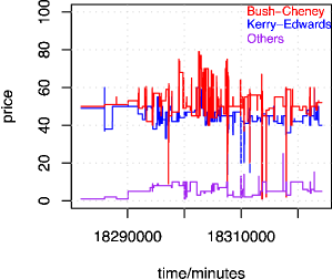
Figure 1: Price time-series for the futures in the 2004 U.S. presidential election. Others represents votes received by all candidates others than Bush-Cheney and Kerry-Edwards.

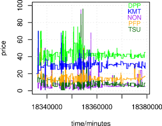
Figure 2: Price time-series for the futures in the 2004 Taiwan parliamentary election. Labels, except NON, are the acronyms of the major political parties participating in the election. NON stands for all candidates other than the four major parties.

Due to the nature of the futures, tournaments were scheduled to start one month before the election day and ended on the election day when the futures matured. Recruiting as many players as possible presented a great challenge to researchers who lacked marketing channels. What was done was to post news about the tournament to college campus bulletin boards throughout TaiwanWang et al. (2004). Numbers of registrations increased with time and reached 364 and 498 respectively for the U.S. presidential and the Taiwan parliamentary election near the end of the tournaments. There was a change in the rules between the two experiments. In the U.S. case, submitted orders waited in the orderbook for matching orders until expired otherwise. In the Taiwan case, orders could be canceled before they expired. Note that contracts could by no means be bought (sold) from (to) oneself. Figures 1 and 2 show the price time-series for each contract in the two experiments. Time is measured in minutes since midnight of January 1, 1970 UTC (coordinated universal time). The higher frequency of trades in the second experiment reflects the change in rules. Our analysis of data thus focuses on the second experiment unless otherwise stated. Interpretation of the price movements and accuracy and precision of the prediction of the time-series on election outcomes are beyond the scope of this paper. We briefly mention here that vote-share rankings by the means of the price time-series correctly mirrored the election outcomes in both experiments, which is also true for our earlier experiment on Taiwan presidential election in March 2004Wang et al. (2004).

III Data Analysis

During the tournament, information arrives stochastically and the time intervals between successive transactions are irregular. To generate a time series at a constant time interval of 1 minute, we bin time into discrete values with a resolution of 1 minute. Prices in a time bin are then averaged. A value of zero, meaning no transactions in that time bin, is replaced with the price in the previous time bin. There are thus a total of 43430 data points in such price time series corresponding to the duration of the tournament in minutes. For volume time series, no such padding is performed, however. Only 8340 nonzero data points were recorded in the volume time series. The ratio of 8340 to 43430 indicates that the market was active 19% of the time.

We call the portfolio consisting of a share of DPP, KMT, NON, PFP, and TSU a bundle. Similar to a stock index which is a (weighted) sum of the stock prices of the representative companies, we sum the five price time-series of the individual futures contracts to obtain the price time-series of a bundle. Figure 3 shows the time-series of the summed prices and summed trading volumes. Hereafter, the analysis will be on such summed observables unless otherwise stated.

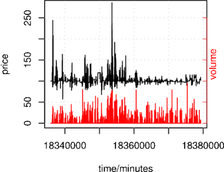
Figure 3: Time-series for the bundle price (black) and total volume (red) for the 2004 Taiwan parliamentary election.

There appear many large fluctuations in Fig. 3. To study occurrence of the fluctuations, we calculate the difference between the logarithmic price $\log S(t)$ at time $t+\tau$ and that at time $t$,

$$G_{\tau}(t)=\log S(t+\tau)-\log S(t),$$ (1)

and the normalized price return,

$$g_{\tau}(t)={G_{\tau}(t)-\mu_{\tau}\over\sigma_{\tau}},$$ (2)

where $\mu_{\tau}$ and $\sigma_{\tau}$ are the mean and standard deviation of $G_{\tau}(t)$. Figure 4 superposes the probability densities of the return $g_{\tau}$ at five different time lags: $\tau=$ 55, 148, 403, 1097 and 8103 minutes, which are roughly evenly spaced in a logarithmic scale. The scaling behavior of price returns over time lags spanning over 2 decades was well documentedMandelbrot (1963); Farma (1965); Dacorogna et al. (1993); Loretan and Phillips (1994); Lux (1996); Pagan (1996); Bouchaud and Potters (Alea-Saclay, Eyrolles, 1998); Arnéodo et al. (1998); Gopikrishnan et al. (1999); Plerou et al. (1999) and reminiscent of the phenomena of self-organized criticality in some physical systemsBak et al. (1987); Field et al. (1995).

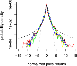
Figure 4: Probability density of normalized price returns with time lag equal to 55 (red), 148 (black), 403 (yellow), 1097 (green) and 8103 (blue) minutes. Dashed line is obtained from a Cauchy distribution and dotted line a Gaussian distribution of unit variance.

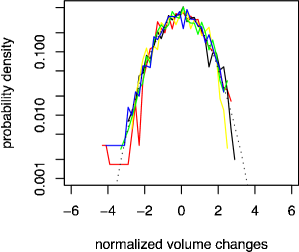
Figure 5: Probability density of normalized volume changes with time lag equal to 55 (red), 148 (black), 403 (yellow), 1097 (green) and 8103 (blue) minutes. Dotted line is obtained from a standardized Gaussian distribution.

Figure 6: Probability density of volume traded (log transformed). The straight line results from a linear regression fit to the large volume data points, giving a slope of -3.9.

In parallel to changes in price, we calculated normalized volume changes and plot the probability densities in Fig. 5, which, unlike the fat tails in Fig. 4, coincides with a standardized normal distribution. The normality indicates that, unlike price fluctuations, volume fluctuations are independentBachelier (1900) over the range of time lags tested.

Another distribution of interest is that of volumesGopikrishnan et al. (2000) which we show in Fig. 6. A straight line fit of the distribution $p_{V}$ for large trading volumes $V$ gives,

$$p_{V}\sim{1\over V^{3.9}}\,.$$ (3)

At the end of the tournament, we liquidated the futures contracts left in players’ accounts, the wealth of which can then be calculated. Recall that every player was allocated an amount of 3100 (units of fictitious money) when his account was opened. If the account wealth remains to be 3100 after liquidation, the account is deemed inactive. To obtain the distribution of wealth, we removed inactive accounts, leaving 319 active ones. The wealth distribution $p_{W}$ of the active accounts is shown in Fig. 7, a linear fit to which suggests a power law distributionPareto (Lausanne, 1897); Zipf (Addison-Wesley 1965),

$$p_{W}\sim{1\over W^{2.1}}\,.$$ (4)

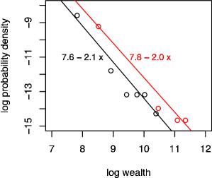
Figure 7: Probability density of wealth (log transformed). The straight lines result from linear regression fits to the whole range of the wealth, giving a slope of about 2. Black and red are, respectively, for the 2004 Taiwan parliamentary and 2004 U.S. presidential election.

IV Discussion

The fat tails in the distribution of price returns have long been observed and suggested to be power-law distributedMandelbrot (1963); Farma (1965); Dacorogna et al. (1993); Loretan and Phillips (1994); Lux (1996); Pagan (1996); Bouchaud and Potters (Alea-Saclay, Eyrolles, 1998); Arnéodo et al. (1998); Gopikrishnan et al. (1999); Plerou et al. (1999). We performed a linear fit to the log transformed probability density of $g_{148}$ for $g_{148}>4$ and obtained an asymptotic density $p_{g_{148}}$ for the normalized returns $g_{148}$,

$$p_{g_{148}}\sim{1\over{g_{148}}^{4.9}}\,.$$ (5)

We note however that the exponent can differ if different constructions of time series are used. In the above, we padded missing prices using the last transaction price. The interpolation is valid under the assumption that players consider the current price fair and thus do not bother to buy or sell. However, one can argue that the lack of transactions only reflects the fact that no one is online during the time bin, rather than an agreement on price among players. We therefore also analyzed the data without padding. In this case, the difference between prices at $t+\tau$ and $t$ can only be formed when both prices exist, resulting in a drop in statistics. Nevertheless, Fig. 8 shows the scaling behavior of the (normalized) price returns thus formed $g^{\prime}_{\tau}$. The exponent of the positive tail of the density of $g^{\prime}_{148}$ is now 3.1,

$$p_{g^{\prime}_{148}}\sim{1\over{g^{\prime}_{148}}^{3.1}}\,.$$ (6)

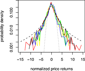
Figure 8: Probability density of normalized returns with time lag equal to 55 (red), 148 (black), 403 (yellow), 1097 (green) and 8103 (blue) minutes. Returns are calculated from the transaction prices. Dashed line is obtained from a Cauchy distribution and dotted line a Gaussian distribution of unit variance.

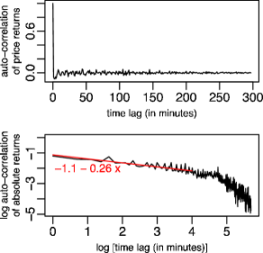
Figure 9: Autocorrelation function of $G_{1}(t)$ (top) and $|G_{1}(t)|$ (bottom). A slope of -0.26 results from a linear regression fit.

The exponents of the price returns are outside the stable Lévy regime. In Fig. 9 is plotted the autocorrelation functions of the price returns and the absolute value of the price returns. Note that data are truncated at time lag equal to 298 minutes, where the first negative autocorrelation of $|G_{1}(t)|$ occurs. It is seen that the autocorrelation of price returns drops to the noise level in about half an hour, after which the market is considered efficient. Higher order correlations however persist longer, as seen in the slow decay of the autocorrelation of the absolute value of the price returns in the bottom panel of Fig. 9, suggesting that traders have long range memories of the magnitude of price changesDing et al. (1983); Dacorogna et al. (1993); Liu et al. (1999).

Our exchange server, which was open 24 hours a day 7 days a week, received orders from online players who submitted their orders in response to random arrivals of information on campaign activities. An order was carried out only when it intersected with a matching order before it expired. When orders were matched, transaction took place. We calculated the time intervals between successive transactions. Figure 10 shows the plot of the numbers of transactions versus inter-transaction time intervals measured in minutes. It is seen that the numbers decay asymptotically in a power-law fashion with an exponent of 1.2. The non-exponentiality of the distribution indicates that transactions do not take place randomly in time, even though orders are assumed to be submitted randomly in time.

Figure 10: Distribution of inter-transaction time intervals (log transformed). The straight line is from a linear regression fit to the data points but the first one, having a slope of -1.2.

A limit order is placed with an upper bound for buying (or lower bound for selling) a volume of shares, expiring in a period of time specified by the bidder (seller). A market order, on the other hand, buys (or sells) from (to) the existing orders in the orderbook, and is executed immediately after it is received on our server. We can therefore say that cautious traders tend to use limit orders while impatient traders use more market orders. The effect of the limit order-limit order interactions and limit order-market order interactions on the price is interesting. Each futures contract has its lowest ask and highest bid price as a function of time. We summed the five time series to form the lowest ask and highest bid time series of the bundle. In Fig. 11 is plotted the time series, which are seen to flank the price time series of Fig. 3. We calculate the arithmetic mean of the lowest ask and highest bid at any time and obtain a time series, the scaling property of which is shown in Fig. 12. The spread of the tails, compared with that in Fig. 4, does not seem to support the exacerbating effect of market orders. However, since the market was thin, players might have learned quickly to avoid placing market orders. More studies are needed to understand the impact of market orders.

In our experiment, an equal amount of money was made available to the market whenever a new player joined the tournament. Players’ money was redistributed via trading as the tournament went on (a player owned on average 11 shares of each contract in the experiment). We showed in Fig. 7 that the distribution of wealth after the 2004 Taiwan parliamentary election is power-law distributed. In the independent experiment on the 2004 U.S. presidential election, we also examined the wealth distribution of the active players (235 in this case) and found a similar exponent for the power law (red line in Fig. 7). The Paretian property appears robust considering the lower changeover rate of the futures contracts in the 2004 U.S. presidential tournament than in the 2004 Taiwan parliamentary tournament (cf. Figs. 1 and 2). The asymptotic fat tailed distribution of price fluctuations also appeared in the 2004 U.S. presidential tournament as we carried out a similar analysis on the time series despite their lower statistics. Formation of the Paretian wealth distributions could be attributed to the large price fluctuations, not the frequency of trades, according to our experiment. To study the effect of different trading rules (social insurance policies) on wealth redistribution, we can, for example, charge a fee (tax) on every transaction (income). We can also study the dynamics by sampling the wealth distribution along the tournament.

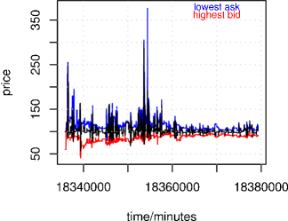
Figure 11: Lowest ask and highest bid time-series of the 2004 Taiwan parliamentary election.

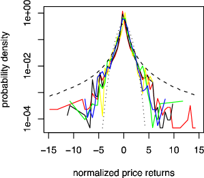
Figure 12: Probability density of normalized price returns with time lag equal to 55 (red), 148 (black), 403 (yellow), 1097 (green) and 8103 (blue) minutes. Returns are calculated from the arithmetic means of lowest asks and highest bids. Dashed line is obtained from a Cauchy distribution and dotted line a Gaussian distribution of unit variance.

A simple survey of the geographical and occupational information on the top 20 players indicates that they do not know one another in person, suggesting that social networks are not necessary to explain the power law property of the price returns and wealth. The decay times in the price autocorrelation functions differ. In particular, the decay time of the DPP price autocorrelation function is found the longest, suggesting that there were more DPP supporters in the tournament or that the DPP supporters were more loyal. Dependencies of the price changes could be caused by the collective actions of segments (coalitions) of participants of different genres, contributing to the large fluctuations.

In summary, we have presented an approach to study the principles underlying complex and strongly fluctuating socioeconomic systems. Futures contracts corresponding to a social event were designed. Futures trading experiments with well defined initial conditions were then set up. Participants were recruited and contributed to the study via the Internet. Market observables such as transaction price, trading volume, bid ask price, were recorded at real time. Scaling behaviors were found in the distributions of price returns and trading volume similar to those found in real financial markets. Power law behaviors were also found in the distributions of inter-transaction time intervals as well as participants’ wealth.

References

- Bachelier (1900) L. Bachelier, Ann. Sci. École Norm. Suppl. 3, 21 (1900).
- Lévy (Gauthier-Villars, Paris, 1937) P. Lévy, Théorie de l’Addition des Variables Aléatoires (Gauthier-Villars, Paris, 1937).
- Mandelbrot (1963) B. B. Mandelbrot, J. Business 36, 294 (1963).
- Farma (1965) E. F. Farma, J. Business 38, 34 (1965).
- Dacorogna et al. (1993) M. M. Dacorogna, U. A. Muller, R. J. Nagler, R. B. Olsen, and O. V. Pictet, J. Int. Money Finance 12, 413 (1993).
- Loretan and Phillips (1994) M. Loretan and P. C. B. Phillips, J. Empirical Finance 1, 211 (1994).
- Lux (1996) T. Lux, Appl. Financial Economics 6, 463 (1996).
- Pagan (1996) A. Pagan, J. Empirical Finance 3, 15 (1996).
- Arnéodo et al. (1998) A. Arnéodo, J.-F. Muzy, and D. Sornette, Eur. Phys. J. B 2, 277 (1998).
- Gopikrishnan et al. (1999) P. Gopikrishnan, V. Plerou, L. A. N. Amaral, M. Meyer, and H. E. Stanley, Phys. Rev. E 60, 5305 (1999).
- Plerou et al. (1999) V. Plerou, P. Gopikrishnan, L. A. N. Amaral, M. Meyer, and H. E. Stanley, Phys. Rev. E 60, 6519 (1999).
- Bouchaud and Potters (Alea-Saclay, Eyrolles, 1998) J. P. Bouchaud and M. Potters, Theorie des Risques Financiéres (Alea-Saclay, Eyrolles, 1998).
- Bak (1992) P. Bak, Physica A 191, 41 (1992).
- Ponzi and Aizawa (2000) A. Ponzi and Y. Aizawa, Physica A 287, 507 (2000).
- Lux and Marchesi (1999) T. Lux and M. Marchesi, Nature 397, 498 (1999).
- Cont and Bouchaud (2000) R. Cont and J. P. Bouchaud, Macroeconomic Dynamics 4, 170 (2000).
- Gabaix et al. (2003) X. Gabaix, P. Gopikrishnan, V. Plerou, and H. E. Stanley, Nature 423, 267 (2003).
- Wang et al. (2004) S. C. Wang, C. Y. Yu, K. P. Liu, and S. P. Li, proceedings of Web Intelligence, IEEE/WIC/ACM International Conference on (WI’04) p. 173 (2004).
- Forsythe et al. (1992) R. Forsythe, F. Nelson, G. R. Neumann, and J. Wright, The Am. Econ. Rev. 82, 1142 (1992).
- Berg and Rietz (2003) J. E. Berg and T. A. Rietz, Information Systems Frontiers p. 79 (2003).
- Smith et al. (2003) E. Smith, J. D. Farmer, L. Gillemot, and S. Krishnamurthy, Quant. Finance 3, 481 (2003).
- Bak et al. (1987) P. Bak, C. Tang, and K. Wiesenfeld, Phys. Rev. Lett. 59, 381 (1987).
- Field et al. (1995) S. Field, J. Witt, and E. Nori, Phys. Rev. Lett. 74, 1206 (1995).
- Gopikrishnan et al. (2000) P. Gopikrishnan, V. Plerou, X. Gabaix, and H. E. Stanley, Phys. Rev. E 62, R4493 (2000).
- Pareto (Lausanne, 1897) V. Pareto, Cours d’économie politique (Lausanne, 1897).
- Zipf (Addison-Wesley 1965) G. K. Zipf, Human behaviour and the principles of least effort (Addison-Wesley 1965).
- Ding et al. (1983) Z. Ding, C. W. J. Granger, and R. F. Engle, J. Empirical Finance 1, 83 (1983).
- Liu et al. (1999) Y. Liu, P. Gopikrishnan, P. Cizeau, M. Meyer, C.-K. Peng, and H. E. Stanley, Phys. Rev. E 60, 1390 (1999).