How Hertzian solitary waves interact with boundaries in a 1-D granular medium

Abstract

We perform measurements, numerical simulations, and quantitative comparisons with available theory on solitary wave propagation in a linear chain of beads without static preconstrain. By designing a nonintrusive force sensor to measure the impulse as it propagates along the chain, we study the solitary wave reflection at a wall. We show that the main features of solitary wave reflection depend on wall mechanical properties. Since previous studies on solitary waves have been performed at walls without these considerations, our experiment provides a more reliable tool to characterize solitary wave propagation. We find, for the first time, precise quantitative agreements.

DOI: 10.1103/PhysRevLett.94.178002

Solitons are widely studied in physics because of their ubiquity in systems exhibiting nonlinear propagation Drazin and Johnson (2002). In a granular chain, theoretical and experimental evidence of solitons was first reported by Nesterenko Nesterenko (1984); Lazaridi and Nesterenko (1985); Gavrilyuk and Nesterenko (1994); Nesterenko (1994); Nesterenko et al. (1995); Nesterenko (2001). Since Nesterenko’s pioneering work, most of the experimental effort in the field has generally focused on the scaling laws for amplitude and speed of the solitons, Coste et al. (1997); Coste and Gilles (1999). It was recently reported Manciu et al. (2001a) that identical and opposite propagating solitons do not preserve themselves upon collision and hence these are solitary waves rather than solitons. Several detailed numerical studies have been devoted to understand the interactions of solitary waves with a perfectly reflecting wall Manciu et al. (2001b, a); Manciu and Sen (2002); Xu and Hong (2001); Hascoet et al. (1999) and show that tiny secondary solitary waves are generated as a solitary wave is reflected off a wall Manciu et al. (2001a); Manciu and Sen (2002). However, due to experimental difficulties, no close comparison between experiments and simulations has so far been established. Here inspired by Nesterenko’s experiments Nesterenko (1994); Nesterenko et al. (1995); Nesterenko (2001), we developed an adapted impulse sensor to nonintrusively investigate solitary wave propagation in a linear chain of identical elastic beads. We explored the problem of solitary wave reflection by changing the elastic properties of the wall and showed that the solitary wave detected at the wall differs from the actual solitary wave propagating through the chain. Our measurements significantly improve upon previous experimental studies  Lazaridi and Nesterenko (1985); Coste et al. (1997) and allows excellent agreement with our numerical simulations and Nesterenko’s analytical theory  Nesterenko (2001).

The physical behavior of solitary waves in bead chains can be described as follows. Under elastic deformation, the energy stored at the contact between two elastic bodies submitted to an axial compression corresponds to the Hertz potential Landau and Lifshitz (1967) $U_{H}=(2/5)\kappa\delta^{5/2}$, where $\delta$ is the overlap deformation between bodies, $\kappa^{-1}=(\theta+\theta^{\prime})(R^{-1}+R^{\prime-1})^{1/2}$, $\theta=3(1-\nu^{2})/(4Y)$, and $R$ and $R^{\prime}$ are radii of curvature at the contact. $Y$ and $\nu$ are Young’s Modulus and Poisson’s ratio, respectively. Since the force felt at the interface is the derivative of the potential with respect to $\delta$, ($F_{H}=\partial_{\delta}U_{H}=\kappa\delta^{3/2}$), the dynamics of the chain of beads is described by the following system of $N$ coupled nonlinear equations,

$$m\partial_{tt}^{2}u_{n}=\kappa\left[(u_{n-1}-u_{n})^{3/2}_{+}-(u_{n}-u_{n+1})^{3/2}_{+}\right],$$ (1)

where $m$ is the mass, $u_{n}$ is the position of the center of mass of bead $n$, $u_{n}=2nR$ at rest, and the label $+$ on the brackets indicates that the Hertz force is zero when the beads lose contact. Under the long-wavelength approximation $\lambda\gg R$ (where $\lambda$ is the characteristic wavelength of the perturbation), the continuum limit of Eq. 1 can be obtained by replacing the discrete function $u_{n\pm 1}(t)$ by the Taylor expansion of the continuous function $u(x\pm 2R,t)$. Keeping terms of up to the fourth order spatial derivatives, Eq. 1 leads to the equation for the strain $\psi=-\partial_{x}u>0$,

$$\partial_{tt}^{2}\psi\simeq c^{2}\partial^{2}_{xx}[\psi^{3/2}+(2/5)R^{2}\psi^{1/4}\partial^{2}_{xx}(\psi^{5/4})],$$ (2)

where $c=(2R)^{5/4}(\kappa/m)^{1/2}$  Nesterenko (2001). Looking for progressive waves with speed $v$, in the form $\psi(\xi=x-vt)$, Eq. 2 admits an exact periodic solution in the form $\psi=(5/4)^{2}\times(v/c)^{4}\cos^{4}[\xi/(R\sqrt{10})]$ Nesterenko (1984); Lazaridi and Nesterenko (1985); Gavrilyuk and Nesterenko (1994); Nesterenko (1994); Nesterenko et al. (1995). Although this solution only satisfies the truncated Eq. 1, there is quantitative analysis on how well one hump ($-\pi/2<\xi/(R\sqrt{10})<\pi/2$) of this periodic function represents a soliton solution  Nesterenko (1984); Chatterjee (1999). Approximating the spatial derivative, the strain in the chain reads $\psi\simeq\delta/(2R)$, and the force felt at beads contact, $F\simeq\kappa(2R\psi)^{3/2}$, and $v$ become,

$$F\simeq F_{m}\cos^{6}{\left[\frac{x-vt}{R\sqrt{10}}\right]};v\simeq\left(\frac{6}{5\pi\rho}\right)^{\frac{1}{2}}\left(\frac{F_{m}}{\theta^{2}R^{2}}\right)^{\frac{1}{6}}.$$ (3)

In our experiment, we consider the chain of $21$ identical beads of mass $m$, located on a Plexiglas linear track as shown on top of Fig. 1. A piezoelectric dynamic impulse sensor (PCB 208A11 with sensitivity $112.40$ mV/N) located at the end of the chain provides the force at the rigid end. This sensor has a flat cap made of the same material as the beads. Beads are Tsubaki high carbon chrome hardened steel roll bearing (norm JIS SUJ2 equivalent to AISI 52100). The radius of the beads is $R=13$ mm (tolerance is $\pm 125$ $\mu$m on diameter), and the density is $\rho=7780$ kg/m³. The Young’s modulus is $Y=203\pm 4$ GPa Tsu , and the Poisson ratio is assumed to be $\nu=0.3$; our beads have thus a $\kappa=12$ N/$\mu$m^3/2. Moreover, the deformation keeps elastic and below yield stress ($\sigma_{Y}=2$ GPa Tsu ). Assuming that the contact surface is a disk of area $A=\pi({\theta}RF)^{2/3}$ Landau and Lifshitz (1967), the corresponding maximum compression force is roughly $F_{Y}\simeq 470$ N, which corresponds to an overlap $\delta_{Y}\simeq 11$ $\mu$m. Forces inside the chain are monitored by a flat dynamic impulse sensor (PCB 200B02 with sensitivity $11.24$ mV/N) that is inserted inside one of the beads, cut in two parts. The total mass of the bead sensor system has been compensated to match the mass of an original bead. This system allows achieving non intrusive force measurement by preserving both contact and inertial properties of the bead-sensor system. The stiffness of the sensor $k_{s}=1.9$ kN/$\mu$m being greater than the stiffness of the Hertzian contact ($k_{s}\gg k_{H}\propto\kappa\delta^{1/2}$), means the coupling between the chain and the sensor is consequently negligible. To relate the force $F_{s}$ registered by the sensor with the actual force at the beads contact, we write the Newton’s law for both masses, respectively, located in front ($+$) and in the back ($-$) of the sensor. Thus, $F_{\pm}=F_{s}\pm m_{\pm}\partial_{tt}^{2}x_{\pm}$, with $F_{s}=k_{s}(x_{+}-x_{-})$. This set of equations can be summarized as

$$\partial_{tt}^{2}F_{s}+\omega_{0}^{2}F_{s}=\omega_{0}^{2}\left[(1-\beta)F_{+}+{\beta}F_{-}\right],$$ (4)

where we have introduced the resonant angular frequency of the system $\omega_{0}=[k_{s}(m_{+}^{-1}+m_{-}^{-1})]^{1/2}$, and the mass ratio $\beta=m_{+}/(m_{+}+m_{-})$. Experimentally $\beta=0.11$ and the resonant frequency, $f_{0}=\omega_{0}/(2\pi)\simeq 85$ kHz, indicates that safe measurements can be obtained for signal whose period is greater than $\tau_{0}=1/f_{0}\simeq 12$ $\mu$s. However, a relation between $F_{\pm}(t)$ is needed to invert Eq. 4 and then determine the force $F_{+}(t)$ or $F_{-}(t)$ from the force $F_{s}(t)$. Assuming that the pulse travels at a velocity $v$, this relation reads $F_{-}(t)=F_{+}(t+t_{0})$, where $t_{0}=(x_{+}-x_{-})/v$. An estimate of the velocity $v$ is obtained from the time of flight of the pulse and the deconvolution of Eq. 4 by means of Fast Fourier Transform, then provides the actual force $F_{+}(t)$ felt exactly at the interface between two beads. Notice that the improvement introduced here represents a correction of the order of $\beta$, i.e. about $10\%$. Signals from sensors are amplified by a conditioner (PCB 482A16), recorded by a two channels numeric oscilloscope (Tektronix TDS340), and transferred to a computer. The acquisition is triggered by the contact between the small impacting bead and the chain; both being in contact with soft wires they cause the discharge of a capacitor in a resistor ($1/RC\simeq 1$ $\mu$s). This circuit allows high repeatability, e.g. for time of flight measurements. In Fig. 1a, a solitary wave propagates along the chain of beads. The central peak corresponds to the impulse detected at the end, whereas the two peaks on the sides are the incident and reflected waves measured inside the chain. Notice that the central peak is much higher and broader than the actual solitary wave propagating along the chain, thus no quantitative information can be extracted from it without a detailed description of the interaction between the solitary wave and the wall. In order to characterize solitary waves, we look both for velocity and duration of incident pulses recorded at one contact far from the wall. According to Eq. 3, we map experiments to $F(t)=F_{m}\cos^{6}[(t-t_{0})/\tau]$, to obtain the amplitude $F_{m}$, the duration $2\tau$, and the time of flight $t_{0}$ of a pulse. To provide more accurate data for the velocity, we perform flight time measurements for different positions of the active bead. In addition, for every experimental configuration we record three sets of data and check repeatability, and the whole experiment is repeated three times. According to Eq. 3, we first look for the best fit in a least squares sense for the experimental velocity of the pulse, in the form $v=CF_{m}^{1/6}$, and we find an experimental value $C_{e}=203.6\pm 8.9$ in standard units. This value agrees with the theoretical prediction $C_{t}=198.9$, derived from Eq. 3, within an error less than $3\%$. The fit is plotted in straight line in Fig. 2a. For sake of comparison, we also plot (the straight line on Fig. 2b) the duration $2\tau=2R\sqrt{10}/v$, also obtained from Eq. 3. The velocity is thus in a satisfactory agreement with the theoretical prediction, which also appears at first glance to predict in a good manner the duration of the pulse. However, energy dissipation is expected to produce a broader solitary wave. Dissipation is characterized by the restitution coefficient (see Fig. 2c) defined as $\epsilon=(U_{n+1}/U_{n})^{1/2}=(F_{n+1}/F_{n})^{5/6}$ ($U_{n}$ is the Hertz potential, i.e., the work done by the Hertz force $F_{n}$ at the contact $n$). Here we consider two mechanisms responsible for the dissipation; internal viscoelasticity and solid friction of beads submitted to their weight $mg$ ($g$ is the gravity), on the track. A third mechanism, the solid friction between beads due to thwarted rotations Duran (1997), may also be taken into account. However, the contribution of a friction force of the form $F_{s}^{*}=\mu^{*}\kappa\delta^{3/2}$ into Eq. 1 reduces simply to considering an equivalent nonlinear stiffness $\kappa^{*}=(1+\mu^{*})\kappa$. Viscoelastic dissipation is included by using the simplest approximation Kuwabara and Kono (1987); Brilliantov et al. (1996) for which the dissipative force at the contact of two beads reads, $F_{v}=\eta\kappa\partial_{t}(\delta^{3/2})$, where $\eta$ includes unknown coefficients due to internal friction of the material Landau and Lifshitz (1967); Brilliantov et al. (1996). Solid friction is taken into account by considering a frictional force $F_{s}=\mu mg$ Duran (1997). The potential energy difference $(U_{n}-U_{n+1})$ being equal to the work done by both previous dissipative forces allows us to estimate the restitution coefficient to be force dependent, $\epsilon=(U_{n+1}/U_{n})^{1/2}\simeq 1-C_{v}F^{1/6}-C_{s}/F$. Simple calculations provide the relation of $\eta$ and $\mu$ with the new constants $C_{v}$ and $C_{s}$ as, $\eta\approx{2\sqrt{10}RC_{v}/5C}$ and $\mu\approx{4C_{s}/5mg}$ respectively. Experimentally, we determine that $C_{v}=1.9\times 10^{-2}$ and $C_{s}=1.7\times 10^{-1}$ in standard units, see Fig. 2c. Then, $\eta_{e}\approx{1.8}$ $\mu$s and $\mu_{e}\approx{0.19}$.

Numerical simulations based on a Velocity-Verlet algorithm allow to explore the main features of solitary waves by solving Eq. 1 directly. We first run numerical calculation without dissipation, plotted in dashed lines on Fig. 2a and 2b. Looking for least square fit for the velocity, as previously done, we find $C_{n}=201.5\pm 0.1$. Compared to the theoretical value $C_{t}$, simulations improve the agreement with experiments (relative error on velocity is about $1\%$), but a noteworthy disagreement is now observed for the duration of the pulse (see Fig. 2b), which is about $10\%$ lower than experimental values. This lag is consistent with the presence of a weak dissipation. At this stage, we only consider the effect of viscoelastic dissipation in numerical simulations. We thus adjust the coefficients, and for $\eta_{n}=2$ $\mu$s and $\mu=0$, a good agreement can be obtained both for the velocity and the duration, in the range of amplitude where viscoelastic dissipation dominates over solid friction ($F_{m}>50$ N). Notice that $\eta_{n}$ differs from the experimental value $\eta_{e}$ only by $20\%$. Since solid friction has not yet been included in simulations, the experimental pulse is still broader than in simulations at low force amplitude ($F_{m}<20$ N) where this mechanism dominates.

We now check how simulations reproduce the features of the reflection process. Figure 1b shows the corresponding numerical simulations for the incident and the reflected solitary wave as well as the force registered at the wall. Although simulations include only viscous dissipation, $\eta_{n}=2$ $\mu$s, the agreement between Fig. 1a and Fig. 1b is very good. Notice that momentum is conserved, i.e., the area of the central peak in Fig. 1a is equal to the area of the incident plus the reflected solitary wave. Figure 1c presents the corresponding calculations of the time evolution of the potential and kinetic energy when a solitary wave interacts with the wall sensor. The solitary wave is initiated at $t=0$ by a purely kinetic impact. At $t=1$ ms the pulse reaches the rigid sensor and the energy is stored into potential. The pulse is then reflected and propagates backward to the free end until leading to ejection of beads after $t=2$ ms.

We further investigated the solitary wave reflection by varying the mechanical properties of the flat part of sensor in contact with the last bead. This is done by locating polished disks of $1$ mm thickness and $5$ mm diameter of different known materials on the active part of the sensor. These samples are made of plexiglass, Mg, Cu, Si, Fe, and W. For materials softer than the beads, unexpected features arise. For instance, in Fig. 3b, the experimental force on the wall exhibits a well defined secondary peak. The break of symmetry implied by the change of elastic properties leads to the generation of a so-called secondary solitary wave in the reflected impulse predicted recently via simulations in Manciu et al. (2001b); Manciu and Sen (2002). Dissipationless numerical simulations in Fig. 3c reproduce well the experimental finding of Fig. 3b without adjustable parameter. Better agreement can be achieved but it requires the knowledge of the mechanism dominating dissipation of the samples. Fig 3a is the ratio of the maximum force measured at the wall and the respective maximum force of the incident solitary wave. Despite the peculiar form of the force, the ratio of maximum forces follows a well defined law that is characteristic of the kinetic to potential energy conversion at the wall. This interesting feature should prove valuable to determine the Young modulus of materials of unknown nature, when the sample size is a practical limitation.

To understand the underlying physics of solitary wave reflection, we focus on the kinetic-potential energy conversion when a solitary wave interacts with a rigid wall. As shown on Fig. 1c and Nesterenko (1984, 2001), when solitary wave propagates freely in the chain, the kinetic energy $K_{chain}$ is about 56% and the potential energy $U_{chain}$ is about 44% of the total energy (for a rough estimation we assume $K_{chain}\simeq U_{chain}$). However, when a solitary wave reaches the end of the chain, the potential energy stored at the sensor-bead contact equals the total energy carried by the solitary wave. The kinetic energy is thus transformed into potential at the contact. Then, $U_{end}^{max}\simeq 2U_{chain}$. On the other hand, the solitary wave extends on a few beads, and the potential energy stored in the chain is roughly supported by the most compressed contact ($U_{chain}\simeq U_{bead}^{max}$). It finally becomes,

$$\frac{U_{end}^{max}}{U_{bead}^{max}}\simeq 2\rightarrow\frac{F_{end}^{max}}{F_{bead}^{max}}\simeq 2^{6/5}\left(1+\frac{Y_{bead}}{Y_{end}}\right)^{-2/5}$$ (5)

which is a function of Young modulus of beads and the sensor plane. In Fig. 3a, we compare experiments, numerical simulation, and the above estimate. Within the error bars, a satisfactory agreement is obtained.

In conclusion, we have developed a non intrusive reliable method to investigate solitary wave propagation and solitary wave reflection at walls. Our measurements in conjunction with our numerical simulations provide a powerful tool to accurately investigate a variety of related problems such as the main features of solitary waves reaching impedance mismatch, the generation of the recently predicted secondary solitary waves at the boundaries, and the solitary wave interactions, among others.

This work received the support of Conicyt under program Fondap No. 11980002. The Consortium of the Americas is acknowledged for supporting the visit of A.S. to Chile. S.S. acknowledges partial support of NSF-CMS-0070055.

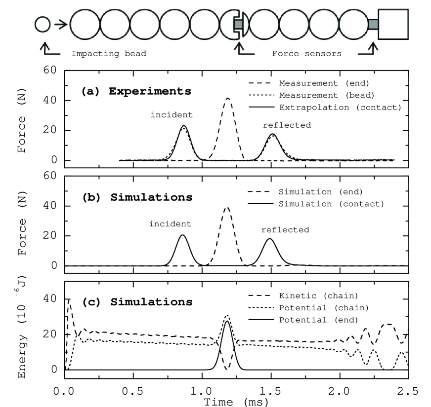
Figure 1: (top) Schematic view of experimental setup. (a) Experiments: middle peak indicates the force signal at the end of the chain, whereas lateral peaks are the incident and reflected solitary wave. The solid line represents the force at a single contact extrapolated from Eq. 4. (b) and (c) The numerical simulations of the contact forces and energy, respectively, for $\eta_{n}=2\mu$s.

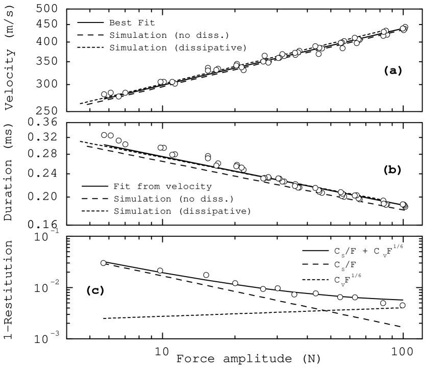
Figure 2: (a) Velocity $v$ and (b) duration $2\tau$ of the solitary wave, measured inside the chain, vs force amplitude. Theoretical predictions from Eq. 3, and numerical simulations are contrasted to experimental data. (c) Restitution coefficient vs force amplitude.

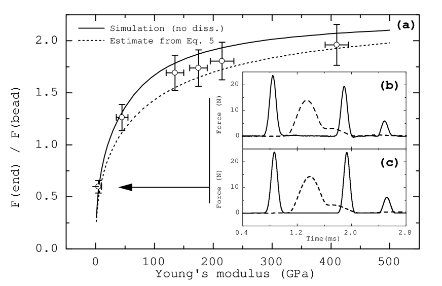
Figure 3: (a) Ratio of force amplitudes at the end of the chain and of the incident impulse vs Young’s modulus of the sample placed on the rigid sensor. Inset (b) force measurements when a solitary wave collides on the softer sample ($Y=5$ GPa), and (c) corresponding simulation reproducing all the experimental features for $\eta_{n}=0$. Dashed lines indicate forces at the end of the chain. The last peaks on the right represent the secondary solitary waves.

References

- Drazin and Johnson (2002) P. G. Drazin and R. S. Johnson, Solitons: An introduction (Cambridge University Press, Cambridge, England, 2002).
- Nesterenko (1984) V. F. Nesterenko, J. Appl. Mech. Tech. Phys. 24, 733 (1984).
- Lazaridi and Nesterenko (1985) A. N. Lazaridi and V. F. Nesterenko, J. Appl. Mech. Tech. Phys. 26, 405 (1985).
- Gavrilyuk and Nesterenko (1994) S. L. Gavrilyuk and V. F. Nesterenko, J. Appl. Mech. Tech. Phys. 34, 784 (1994).
- Nesterenko (1994) V. F. Nesterenko, J. Phys. IV 4, C8 (1994).
- Nesterenko et al. (1995) V. F. Nesterenko, A. N. Lazaridi, and E. B. Sibiryakov, J. Appl. Mech. Tech. Phys. 36, 166 (1995).
- Nesterenko (2001) V. F. Nesterenko, Dynamics of heterogeneous materials (Springer-Verlag, New York, 2001).
- Coste et al. (1997) C. Coste, E. Falcon, and S. Fauve, Phys. Rev. E 56, 6104 (1997).
- Coste and Gilles (1999) C. Coste and B. Gilles, Eur. Phys. J. B 7, 155 (1999).
- Manciu et al. (2001a) M. Manciu, S. Sen, and A. J. Hurd, Physica D (Amsterdam) 157, 226 (2001a).
- Manciu et al. (2001b) M. Manciu, S. Sen, and A. J. Hurd, Phys. Rev. E 63, 016614 (2001b).
- Manciu and Sen (2002) F. S. Manciu and S. Sen, Phys. Rev. E 66, 016616 (2002).
- Xu and Hong (2001) A. G. Xu and J. Hong, Commun. Theor. Phys. 35, 106 (2001).
- Hascoet et al. (1999) E. Hascoet, H. J. Hermann, and V. Loreto, Phys. Rev. E 59, 3202 (1999).
- Landau and Lifshitz (1967) L. D. Landau and E. M. Lifshitz, Theorie de l’élasticité (Mir, Moscou, 1967), 2nd ed., in French.
- Chatterjee (1999) A. Chatterjee, Phys. Rev. E 59, 005912 (1999).
- (17) See, for instance, http://www.wsb.co.th/.
- Duran (1997) J. Duran, Sables, Poudres et Grains (Eyrolles, Paris, 1997).
- Kuwabara and Kono (1987) G. Kuwabara and K. Kono, Jpn. J. Appl. Phys. 26, 1230 (1987).
- Brilliantov et al. (1996) N. V. Brilliantov, F. Spahn, J. M. Hertzsch, and T. Pöschel, Phys. Rev. E 53, 5382 (1996).