Lattice Boltzmann Model for Axisymmetric Multiphase Flows

Abstract

In this paper, a lattice Boltzmann (LB) model is presented for axisymmetric multiphase flows. Source terms are added to a two-dimensional standard lattice Boltzmann equation (LBE) for multiphase flows such that the emergent dynamics can be transformed into the axisymmetric cylindrical coordinate system. The source terms are temporally and spatially dependent and represent the axisymmetric contribution of the order parameter of fluid phases and inertial, viscous and surface tension forces. A model which is effectively explicit and second order is obtained. This is achieved by taking into account the discrete lattice effects in the Chapman-Enskog multiscale analysis, so that the macroscopic axisymmetric mass and momentum equations for multiphase flows are recovered self-consistently. The model is extended to incorporate reduced compressibility effects. Axisymmetric equilibrium drop formation and oscillations, breakup and formation of satellite droplets from viscous liquid cylindrical jets through Rayleigh capillary instability and drop collisions are presented. Comparisons of the computed results with available data show satisfactory agreement.

I Introduction

Fluid flow with interfaces and free surfaces is common in nature and in many engineering applications. Such interfacial flows which typically involve multiple scales remain a formidable non-linear problem rich in physics and continue to pose challenges to experimentalists and theoreticians alike Eggers (1997). Numerical simulation of multiphase flows is challenging as the shape and location of the interfaces must be computed in conjunction with the solution of the flow field Hyman (1984); Scardovelli and Zaleski (1999). Computational methods based on the lattice Boltzmann equation (LBE) for simulating complex emergent physical phenomena have attracted much attention in recent years Chen and Doolen (1998); Succi et al. (2002). The LBE simulates multiphase flows by incorporating interfacial physics at scales smaller than macroscopic scales. Phase segregation and interfacial fluid dynamics can be simulated by incorporating inter-particle potentials Shan and Chen (1993, 1994), concepts based on free energy Swift et al. (1995, 1996) or kinetic theory of dense fluids He et al. (1998a, 1999a); He and Doolen (2002).

The formulation of the standard LBE is based on the Cartesian coordinate system and does not take into account axial symmetry that may exist. Numerous multiphase flow situations exist where the fluid dynamics can be approximated as axisymmetric Sussman and Smereka (1996); Eggers (1997). Examples include head-on collision of drops, normal drop impingement on solid surfaces and Rayleigh instability of cylindrical liquid columns. Currently, full three-dimensional (3D) calculations have to be carried out for problems which may be approximated as axisymmetric He et al. (1999b); Inamuro et al. (2003); Premnath and Abraham (2004a). In 3D computations, computational considerations restrict the numerical resolution that may be employed and the physics may not be well resolved. For example, in breakup of drops into satellite droplets the size of the droplets may be such that the 3D grids may not resolve them. To improve the computational efficiency of the LBE for axisymmetric multiphase flows, we propose an axisymmetric LB model in this paper. The approach consists of adding source terms to the two-dimensional (2D) Cartesian LBE model based on the kinetic theory of dense fluids for multiphase flows He et al. (1998a, 1999a). This approach is similar in spirit to the idea proposed in Halliday et al. (2001) to solve single-phase axisymmetric flows. However, multiphase flow problems involve additional complexity as a result of interfacial physics involved, i.e. the surface tension forces and the need to track the interfaces. In this case, the accuracy of the numerical discretization of the source terms representing interfacial physics also becomes an important consideration.

This paper is organized as follows. In Section II, the axisymmetric LBE multiphase model is described. Then, in Section III, its extension to simulate axisymmetric multiphase flows with reduced compressibility effects is described. The computational methodology adopted is also discussed in this section. In Section IV, the axisymmetric model is applied to benchmark problems to evaluate its accuracy. Finally, the paper closes with summary in Section V.

II Axisymmetric LBE Multiphase Flow Model

To simulate axisymmetric multiphase flows, axisymmetric contributions of the order parameter, and inertial, viscous and surface tension forces may be introduced to the standard 2D LBE. The source terms, which will be shown to be spatially and temporally dependent, are determined by performing a Chapman-Enskog multiscale analysis in such a way that the macroscopic mass and momentum equations for multiphase flows are recovered self-consistently. The introduction of source terms makes it necessary to calculate additional spatial gradients when compared to those in the standard LBE. While this approach is developed for a specific LBE multiphase flow model based on kinetic theory of dense fluids He et al. (1998a, 1999a), it can be readily extended to other LBE multiphase flow models.

The governing continuum equations of isothermal multiphase flow Nadiga and Zaleski (1996); Zou and He (1999) in the cylindrical coordinate system when the axisymmetric assumption is employed are

$$\partial_{t}\rho+\frac{1}{r}\partial_{r}\left(\rho ru_{r}\right)+\partial_{z}\left(\rho u_{z}\right)=0,$$ (1)

$$\rho\left(\partial_{t}u_{r}+u_{r}\partial_{r}u_{r}+u_{z}\partial_{z}u_{r}\right)=-\partial_{r}P+F_{s,r}+F_{ext,r}+\frac{1}{r}\partial_{r}\left(r\Pi_{rr}\right)+\partial_{z}\left(\Pi_{rz}\right),$$ (2)

$$\rho\left(\partial_{t}u_{z}+u_{r}\partial_{r}u_{z}+u_{z}\partial_{z}u_{z}\right)=-\partial_{z}P+F_{s,z}+F_{ext,z}+\frac{1}{r}\partial_{r}\left(r\Pi_{zr}\right)+\partial_{z}\left(\Pi_{zz}\right),$$ (3)

where $\rho$ is the density and $u_{r}$ and $u_{z}$ are the radial and axial components of velocity. These equations are derived from kinetic theory that incorporates intermolecular interactions forces which are modeled as a function of density following the work of van der Waals Rowlinson and Widom (1982). The exclusion volume effect of Enskog Chapman and Cowling (1964) is also incorporated to account for increase in collision probability due to the increase in the density of non-ideal fluids. These features naturally give rise to surface tension and phase segregation effects. The other variables which appear in the above equations will now be described. $\Pi_{rr}$, $\Pi_{rz}$, $\Pi_{zz}$ are the components of the viscous stress tensor and are given by

$$\Pi_{rr} = 2\mu\partial_{r}u_{r},$$ (4)

$$\Pi_{rz} = \Pi_{zr}=\mu\left(\partial_{z}u_{r}+\partial_{r}u_{z}\right),$$ (5)

$$\Pi_{zz} = 2\mu\partial_{z}u_{z},$$ (6)

where $\mu$ is the dynamic viscosity. $F_{s,r}$ and $F_{s,z}$ are the axial and radial components respectively of the surface tension force, which are given by Zou and He (1999)

$$F_{s,r} = \kappa\rho\partial_{r}\left[\frac{1}{r}\partial_{r}(r\partial_{r}\rho)+\partial_{z}(\partial_{z}\rho)\right],$$ (7)

$$F_{s,z} = \kappa\rho\partial_{z}\left[\frac{1}{r}\partial_{r}(r\partial_{r}\rho)+\partial_{z}(\partial_{z}\rho)\right],$$ (8)

where $\kappa$ controls the strength of the surface tension force. This parameter is related to the surface tension of the fluid, $\sigma$, through the density gradient across the interface by the equation Evans (1979)

$$\sigma=\kappa\int\left(\frac{\partial\rho}{\partial n}\right)^{2}dn.$$ (9)

Thus, the surface tension is a function of both the parameter $\kappa$ and the density profile across the interface. The terms $F_{ext,r}$ and $F_{ext,z}$ in Eqs. (2) and (3) respectively are the radial and axial components of external forces such as gravity.

The pressure, $P$, is related to density through the Carnahan-Starling-van der Waals equation of state (EOS) Carnahan and Starling (1969)

$$P=\rho RT\left\{\frac{1+\gamma+\gamma^{2}-\gamma^{3}}{(1-\gamma)^{3}}\right\}-a\rho^{2},$$ (10)

where $\gamma=b\rho/4$. The parameter $a$ is related to the intermolecular pair-wise potential and $b$ to the effective diameter of the molecule, $d$, and the mass of a single molecule, $m$, by $b=2\pi d^{3}/3m$. $R$ is a gas constant and $T$ is the temperature. The Carnahan-Starling EOS has a supernodal $P-1/\rho-T$ curve, i.e., $dP/d\rho<0$, for certain range of values of $\rho$, when the state fluid temperature is below its critical value. This unstable part of the curve is the driving mechanism responsible for keeping the phases of fluids segregated and for maintaining a self-generated sharp interface.

We now modify the standard LBE in such a way that it effectively yields the axisymmetric multiphase flow equations, Eqs. (1)- (10), in a self-consistent way. To facilitate this, we employ the following coordinate transformation, illustrated in Fig. 1, which allows the governing equations to be represented in a Cartesian-like coordinate system, i.e. $(x,y)$:

Figure 1: Schematic of arrangement of coordinate system in axisymmetric multiphase flow ($(r,z)$ and $(y,x)$ coordinate directions are shown).

$$(r,z)\rightarrow(y,x),$$ (11)

$$(u_{r},u_{z})\rightarrow(u_{y},u_{x}).$$ (12)

Assuming summation convention for repeated subscript indices, Eqs. (1)-(8) may be transformed to

$$\partial_{t}\rho+\partial_{k}\left(\rho u_{k}\right)=-\frac{\rho u_{y}}{y},$$ (13)

$$\rho\left(\partial_{t}u_{i}+u_{k}\partial_{k}u_{i}\right)=-\partial_{i}P+F_{s,i}+F_{ext,i}+\partial_{k}\left[\mu\left(\partial_{k}u_{i}+\partial_{i}u_{k}\right)\right]+F_{ax,i},$$ (14)

where

$$F_{s,i}=\kappa\rho\partial_{i}\nabla^{2}\rho$$ (15)

and $i,j,k\in\left\{x,y\right\}$. The right hand side (RHS) in Eq. (13), $-\rho u_{y}/y$, is the additional term in the continuity equation that arises from axisymmetry. The corresponding term for the momentum equation, Eq. (14), is

$$F_{ax,i}=\frac{\mu}{y}\left[\partial_{y}u_{i}+\partial_{i}u_{y}\right]+\kappa\rho\partial_{i}\left(\frac{1}{y}\partial_{y}\rho\right).$$ (16)

To recover Eqs. (13) and (14), we introduce two additional source terms, $S_{\alpha}^{{}^{\prime}}$ and $S_{\alpha}^{{}^{\prime\prime}}$, to the standard 2D Cartesian LBE which has $\Omega_{\alpha}$ as its collision term and a source term for the internal and external forces, $S_{\alpha}$. These unknown additional terms, representing the axisymmetric mass and momentum contributions respectively, are to be determined so that the macroscopic behavior of the proposed LBE corresponds to axisymmetric multiphase flow. Thus, we propose the following LBE

$$f_{\alpha}(\mbox{\boldmath$x$}+\mbox{\boldmath$e$}_{\alpha}\delta_{t},t+\delta_{t})-f_{\alpha}(\mbox{\boldmath$x$},t) = \frac{1}{2}\left[\Omega_{\alpha}|_{(x,t)}+\Omega_{\alpha}|_{(x+e_{\alpha}\delta_{t},t+\delta_{t})}\right]+$$ (17)

$$\frac{1}{2}\left[S_{\alpha}|_{(x,t)}+S_{\alpha}|_{(x+e_{\alpha}\delta_{t},t+\delta_{t})}\right]\delta_{t}+$$

$$\frac{1}{2}\left[S_{\alpha}^{{}^{\prime}}|_{(x,t)}+S_{\alpha}^{{}^{\prime}}|_{(x+e_{\alpha}\delta_{t},t+\delta_{t})}\right]\delta_{t}+$$

$$\frac{1}{2}\left[S_{\alpha}^{{}^{\prime\prime}}|_{(x,t)}+S_{\alpha}^{{}^{\prime\prime}}|_{(x+e_{\alpha}\delta_{t},t+\delta_{t})}\right]\delta_{t},$$

where $f_{\alpha}$ is the discrete single-particle distribution function, corresponding to the particle velocity, $\mbox{\boldmath$e$}_{\alpha}$, where $\alpha$ is the velocity direction. The Cartesian component of the particle velocity, $c$, is given by $c=\delta_{x}/\delta_{t}$, where $\delta_{x}$ is the lattice spacing and $\delta_{t}$ is the time step corresponding to the two-dimensional, nine-velocity model(D2Q9) Qian et al. (1992) shown in Fig. 1. Here, the collision term is given by the BGK approximation Bhatnagar et al. (1954)

$$\Omega_{\alpha}=-\frac{f_{\alpha}-f_{\alpha}^{eq}}{\tau},\quad\tau=\frac{\lambda}{\delta_{t}},$$ (18)

where $\lambda$ is the relaxation time due to collisions, $\delta_{t}$ is the time step and $f_{\alpha}^{eq}$ is the truncated discrete form of the Maxwellian

$$f_{\alpha}^{eq}\equiv f_{\alpha}^{eq,M}(\rho,\mbox{\boldmath$u$})=\omega_{\alpha}\left\{1+\frac{\mbox{\boldmath$e$}_{\alpha}\cdotp\mbox{\boldmath$u$}}{RT}+\frac{\left(\mbox{\boldmath$e$}_{\alpha}\cdotp\mbox{\boldmath$u$}\right)^{2}}{2(RT)^{2}}-\frac{1}{2}\frac{\mbox{\boldmath$u$}\cdotp\mbox{\boldmath$u$}}{RT}\right\},$$ (19)

where $R$ is the gas constant, $T$ is the temperature and $w_{\alpha}$ is the weighting coefficients in the Gauss-Hermite quadrature to represent the kinetic moment integrals of the distribution functions exactly He and Luo (1997a). For isothermal flows, the factor $RT$ is related to the particle speed $c$ as $RT=1/3c^{2}$. The term in Eq. (17)

$$S_{\alpha}=\frac{(e_{\alpha j}-u_{j})(F_{j}+F_{ext,j})}{\rho RT}f_{\alpha}^{eq,M}(\rho,\mbox{\boldmath$u$})$$ (20)

represents the effect of internal and external forcing terms on the change in the distribution function. The internal force term gives rise to surface tension and phase segregation effects which are given by

$$F_{j}=-\partial_{j}\psi+F_{s,j},$$ (21)

where the function $\psi=P-\rho RT$ is the non-ideal part of the equation of state given in Eq. (10). The first two terms on the RHS of Eq. (17) corresponds to those presented by He et al. (1998). As mentioned above, the last two terms, $S_{\alpha}^{{}^{\prime}}$ and $S_{\alpha}^{{}^{\prime\prime}}$, in this equation is to be selected such that its behavior in the continuum limit would simulate the influence of the non-Cartesian-like terms in Eqs. (13) and (14) in a self-consistent way. Since the zeroth kinetic moment of the term $f_{\alpha}^{eq,M}(\rho,0)$ is involved in the derivation of the macroscopic mass conservation equation from the LBE, the source term $S_{\alpha}^{{}^{\prime}}$ in Eq. (17) is proposed to be equal to $f_{\alpha}^{eq,M}(\rho,0)$ multiplied by an unknown $m^{{}^{\prime}}$ and normalized by the density $\rho$. The other source term $S_{\alpha}^{{}^{\prime\prime}}$ is proposed analogous to the source term in Eq.(20). Thus, we propose

$$S_{\alpha}^{{}^{\prime}} = \frac{f_{\alpha}^{eq,M}(\rho,0)}{\rho}m^{{}^{\prime}},$$ (22)

$$S_{\alpha}^{{}^{\prime\prime}} = \frac{(e_{\alpha j}-u_{j})F_{j}^{{}^{\prime\prime}}}{\rho RT}f_{\alpha}^{eq,M}(\rho,\mbox{\boldmath$u$}).$$ (23)

Here the unknowns, $m^{{}^{\prime}}$ and $F_{j}^{{}^{\prime\prime}}$, in the above two equations can be determined through Chapman-Enskog analysis as will be shown later. It must be stressed that all terms, including the collision term, on the RHS are discretized by the application of the trapezoidal rule, since it has been argued that at least a second-order treatment of the source terms is necessary for simulation of multiphase flow He et al. (1998a, 1999a). The macroscopic fields are given by

$$\rho = \sum_{\alpha}f_{\alpha},$$ (24)

$$\rho u_{i} = \sum_{\alpha}f_{\alpha}e_{\alpha i}.$$ (25)

In this model, the order parameter is the density, $\rho$, which distinguishes the different phases in the flow.

Equation (17) is implicit in time. To remove implicitness in this equation we introduce a transformation following the procedure described by He and others He et al. (1998a, b), whereby

$$\bar{f}_{\alpha}=f_{\alpha}-\frac{1}{2}\Omega_{\alpha}-\frac{1}{2}\left(S_{\alpha}+S_{\alpha}^{{}^{\prime}}+S_{\alpha}^{{}^{\prime\prime}}\right)\delta_{t}$$ (26)

in Eq. (17), so that we obtain

$$\bar{f}_{\alpha}(\mbox{\boldmath$x$}+\mbox{\boldmath$e$}_{\alpha}\delta_{t},t+\delta_{t})-\bar{f}_{\alpha}(\mbox{\boldmath$x$},t)=\bar{\Omega}_{\alpha}|_{(x,t)}+\frac{\tau}{\tau+1/2}\left[S_{\alpha}+S_{\alpha}^{{}^{\prime}}+S_{\alpha}^{{}^{\prime\prime}}\right]|_{(x,t)}\delta_{t},$$ (27)

where

$$\bar{\Omega}_{\alpha}=-\frac{\bar{f}_{\alpha}-f_{\alpha}^{eq}}{\tau+1/2}.$$ (28)

Thus, $\bar{f}_{\alpha}$ is the transformed distribution function that removes implicitness in the proposed LBE, Eq. (17), which describes the evolution of the $f_{\alpha}$ distribution function. The following constraints on the equilibrium distribution and the various source terms Luo (2000); Guo et al. (2002) are imposed from their definition:

$$\sum_{\alpha}f_{\alpha}^{eq}=\rho,\quad\sum_{\alpha}f_{\alpha}^{eq}e_{\alpha i}=\rho u_{i},\quad\sum_{\alpha}f_{\alpha}^{eq}e_{\alpha i}e_{\alpha j}=\rho RT\delta_{ij}+\rho u_{i}u_{j},$$

$$\sum_{\alpha}f_{\alpha}^{eq}e_{\alpha i}e_{\alpha j}e_{\alpha k}=\rho(RT)^{2}\left(u_{i}\delta_{jk}+u_{j}\delta_{ki}+u_{k}\delta_{ij}\right),$$ (29)

$$\sum_{\alpha}S_{\alpha}=0,\quad\sum_{\alpha}S_{\alpha}e_{\alpha i}=F_{i},\quad\sum_{\alpha}S_{\alpha}e_{\alpha i}e_{\alpha j}=(F_{i}+F_{ext,i})u_{j}+(F_{j}+F_{ext,j})u_{i},$$ (30)

$$\sum_{\alpha}S_{\alpha}^{{}^{\prime}}=m^{{}^{\prime}},\quad\sum_{\alpha}S_{\alpha}^{{}^{\prime}}e_{\alpha i}=0,\quad\sum_{\alpha}S_{\alpha}^{{}^{\prime}}e_{\alpha i}e_{\alpha j}=m^{{}^{\prime}}RT\delta_{ij},$$ (31)

$$\sum_{\alpha}S_{\alpha}^{{}^{\prime\prime}}=0,\quad\sum_{\alpha}S_{\alpha}^{{}^{\prime\prime}}e_{\alpha i}=F_{i}^{{}^{\prime\prime}},\quad\sum_{\alpha}S_{\alpha}^{{}^{\prime\prime}}e_{\alpha i}e_{\alpha j}=(F_{i}^{{}^{\prime\prime}}u_{j}+F_{j}^{{}^{\prime\prime}}u_{i}).$$ (32)

Then the following relationships are obtained between the transformed distribution function and the macroscopic fields, which also include the curvature effects resulting from axial symmetry:

$$\rho = \sum_{\alpha}\bar{f}_{\alpha}+\frac{1}{2}m^{{}^{\prime}}\delta_{t},$$ (33)

$$\rho u_{i} = \sum_{\alpha}\bar{f}_{\alpha}e_{\alpha i}+\frac{1}{2}(F_{i}+F_{ext,i}+F_{i}^{{}^{\prime\prime}})\delta_{t}.$$ (34)

Now, to establish the unknowns $m^{{}^{\prime}}$ and $F_{j}^{{}^{\prime\prime}}$ in the above formulation, the Chapman-Enskog multiscale analysis is performed Chapman and Cowling (1964). Introducing the expansions He and Luo (1997b)

$$\bar{f}_{\alpha}(\mbox{\boldmath$x$}+\mbox{\boldmath$e$}_{\alpha}\delta_{t},t+\delta_{t}) = \sum_{\alpha=0}^{\infty}D_{t_{n}}\bar{f}_{\alpha}(\mbox{\boldmath$x$},t),$$ (35)

$$D_{t_{n}} \equiv \partial_{t_{n}}+e_{\alpha k}\partial_{k},$$ (36)

$$f_{\alpha} = \sum_{\alpha=0}^{\infty}\epsilon^{n}f_{\alpha}^{(n)},$$ (37)

$$\partial_{t} = \sum_{\alpha=0}^{\infty}\epsilon^{n}\partial_{t_{n}},$$ (38)

where $\epsilon=\delta_{t}$ in Eq. (27) and using Eq. (26) to transform $\bar{f}_{\alpha}$ back to $f_{\alpha}$, the following equations are obtained in the consecutive order of the parameter $\epsilon$:

$$O(\epsilon^{0}):f_{\alpha}^{(0)} = f_{\alpha}^{eq},$$ (39)

$$O(\epsilon^{1}):D_{t_{0}}f_{\alpha}^{(0)} = -\frac{1}{\tau}f_{\alpha}^{(1)}+S_{\alpha}+S_{\alpha}^{{}^{\prime}}+S_{\alpha}^{{}^{\prime\prime}},$$ (40)

$$O(\epsilon^{2}):\partial_{t_{1}}f_{\alpha}^{(0)}+D_{t_{0}}f_{\alpha}^{(1)} = -\frac{1}{\tau}f_{\alpha}^{(2)}.$$ (41)

Now, invoking the Chapman-Enskog ansatz

$$\sum_{\alpha}\left(\begin{array}[]{c}1\\ e_{\alpha i}\end{array}\right)f_{\alpha}^{(0)}=\left(\begin{array}[]{c}\rho\\ \rho u_{i}\end{array}\right),\sum_{\alpha}\left(\begin{array}[]{c}1\\ e_{\alpha i}\end{array}\right)f_{\alpha}^{(n)}=\left(\begin{array}[]{c}0\\ 0\end{array}\right),n\geq 1$$ (42)

and performing $\sum_{\alpha}(\cdotp)$ on Eqs. (40) and (41), we obtain

$$\partial_{t_{0}}\rho+\partial_{k}(\rho u_{k}) = m^{{}^{\prime}},$$ (43)

$$\partial_{t_{1}}\rho = 0,$$ (44)

respectively. Combining the first- and second- order results given by Eqs. (43) and (44) and considering $\partial_{t}=\partial_{t_{0}}+\epsilon\partial_{t_{1}}$, we get

$$\partial_{t}\rho+\partial_{k}(\rho u_{k})=m^{{}^{\prime}}.\\$$ (45)

Comparing this equation and Eq. (13), the unknown $m^{{}^{\prime}}$ is obtained as

$$m^{{}^{\prime}}=-\frac{\rho u_{y}}{y}.\\$$ (46)

This is the axisymmetric contribution to the Cartesian form of the equation for the order parameter, i.e., density characterizing the different phases of the flow. Taking the first kinetic moment, $\sum_{\alpha}e_{\alpha i}(\cdotp)$, of Eqs. (40) and (41), respectively, we get

$$\partial_{t_{0}}(\rho u_{i})+\partial_{k}(\rho u_{i}u_{k}) = -\partial_{i}(\rho RT)+F_{i}+F_{ext,i}+F_{i}^{{}^{\prime\prime}},$$ (47)

$$\partial_{t_{1}}(\rho u_{i})+\partial_{k}\Pi_{ij}^{(1)} = 0,$$ (48)

where

$$\Pi_{ij}^{(1)}=\sum_{\alpha}f_{\alpha}^{(1)}e_{\alpha i}e_{\alpha j}.$$ (49)

Employing the expression for $f_{\alpha}^{(1)}$ from Eq. (40) in Eq. (49), together with the summational constraints given above, and neglecting terms of the order $O(Ma^{3})$ or higher, we get

$$\Pi_{ij}^{(1)}=-\tau RT\rho(\partial_{j}u_{i}+\partial_{i}u_{j}).$$ (50)

Equation (48) then simplifies to

$$\partial_{t_{1}}(\rho u_{i})=\partial_{j}\left(\tau RT\rho(\partial_{j}u_{i}+\partial_{i}u_{j})\right).$$ (51)

Combining Eqs. (47) and (51), we get

$$\partial_{t}(\rho u_{i})+\partial_{k}(\rho u_{i}u_{k})=-\partial_{i}(\rho RT)+F_{i}+F_{ext,i}+F_{i}^{{}^{\prime\prime}}+\partial_{j}\left(\tau\delta_{t}RT\rho(\partial_{j}u_{i}+\partial_{i}u_{j})\right),$$ (52)

or substituting for $F_{i}$ from Eq. (21), we obtain

$$\partial_{t}(\rho u_{i})+\partial_{k}(\rho u_{i}u_{k})=-\partial_{i}P+F_{s,i}+F_{ext,i}+F_{i}^{{}^{\prime\prime}}+\partial_{j}\left(\tau\delta_{t}RT\rho(\partial_{j}u_{i}+\partial_{i}u_{j})\right).$$ (53)

Using Eqs. (45) and (53), this can be simplified to

$$\rho\left(\partial_{t}u_{i}+u_{k}\partial_{k}u_{i}\right)-\frac{\rho u_{i}u_{y}}{y} = -\partial_{i}P+F_{s,i}+F_{ext,i}+F_{i}^{{}^{\prime\prime}}+$$ (54)

$$\partial_{j}\left(\tau\delta_{t}RT\rho(\partial_{j}u_{i}+\partial_{i}u_{j})\right).$$

Comparing Eqs. (14) and (54), we obtain the other unknown $F_{i}^{{}^{\prime\prime}}$ where

$$F_{i}^{{}^{\prime\prime}}=F_{ax,i}-\frac{\rho u_{i}u_{y}}{y}=\frac{\mu}{y}\left[\partial_{y}u_{i}+\partial_{i}u_{y}\right]+\kappa\rho\partial_{i}\left(\frac{1}{y}\partial_{y}\rho\right)-\frac{\rho u_{i}u_{y}}{y}.$$ (55)

This is the axisymmetric contribution to the Cartesian form of the equation for the momentum, where the first, second and the third terms on the RHS correspond to the viscous, surface tension and inertial force contributions, respectively. The dynamic viscosity is related to the relaxation time for collisions by $\mu=\rho\tau\delta_{t}RT=\rho\lambda c_{s}^{2}$, where $c_{s}^{2}=1/3c^{2}$. The set of equations corresponding to the axisymmetric LBE multiphase flow model is given by Eqs. (27) and (28) together with Eqs. (20), (22) and (23), (33) and (34), and (46) and (55). In general, this multiphase model and that proposed by He and others He et al. (1998a) face difficulties for fluids far from the critical point and/or in the presence of external forces. This difficulty is related to the calculation of the intermolecular force in Eq.(21), involving the computation of $\partial_{j}\psi$ which can become quite large across interfaces. Unless this term is accurately computed, the model may become unstable because of numerical errors He et al. (1999b); He (2004). Hence, an improved treatment of this term is necessary. This will now be described.

III Axisymmetric LBE Multiphase Flow Model with Reduced Compressibility Effects

He and co-workers He et al. (1999a) have proposed that through a suitable transformation of the distribution function, $f_{\alpha}$, which involves invoking the incompressibility condition of the fluid, and employing a new distribution function for capturing the interface, the difficulty with handling the intermolecular force term, $\partial_{j}\psi$, can be reduced. We apply this idea to the axisymmetric model developed in the previous section. We replace the distribution function $f_{\alpha}$ by another distribution function $g_{\alpha}$ through the transformation He et al. (1999a)

$$g_{\alpha}=f_{\alpha}RT+\psi(\rho)\frac{f_{\alpha}^{eq,M}(\rho,0)}{\rho}.$$ (56)

The effect of this transformation will be discussed in greater detail below. By considering the fluid to be incompressible, i.e.

$$\frac{d}{dt}\psi(\rho)=\left(\partial_{t}+u_{k}\partial_{k}\right)\psi(\rho)=0,$$ (57)

and using the transformation Eqs. (56) and (26), Eq. (27) is replaced by

$$\bar{g}_{\alpha}(\mbox{\boldmath$x$}+\mbox{\boldmath$e$}_{\alpha}\delta_{t},t+\delta_{t})-\bar{g}_{\alpha}(\mbox{\boldmath$x$},t)=\bar{\Omega}_{g\alpha}|_{(x,t)}+\frac{\tau}{\tau+1/2}\left[S_{g\alpha}+S_{g\alpha}^{{}^{\prime}}+S_{g\alpha}^{{}^{\prime\prime}}\right]|_{(x,t)}\delta_{t},$$ (58)

where

$$\bar{\Omega}_{g\alpha}=-\frac{\bar{g}_{\alpha}-g_{\alpha}^{eq}}{\tau+1/2},$$ (59)

and

$$g_{\alpha}^{eq}=f_{\alpha}^{eq}RT+\psi(\rho)\frac{f_{\alpha}^{eq,M}(\rho,0)}{\rho}.$$ (60)

The corresponding source terms become

$$S_{g\alpha} = (e_{\alpha j}-u_{j})\times$$ (61)

$$\left[(F_{j}+F_{ext,j})\frac{f_{\alpha}^{eq,M}(\rho,\mbox{\boldmath$u$})}{\rho}-\left(\frac{f_{\alpha}^{eq,M}(\rho,\mbox{\boldmath$u$})}{\rho}-\frac{f_{\alpha}^{eq,M}(\rho,0)}{\rho}\right)\partial_{j}\psi(\rho)\right],$$

$$S_{g\alpha}^{{}^{\prime}}=S_{\alpha}^{{}^{\prime}}RT=\frac{f_{\alpha}^{eq,M}(\rho,0)}{\rho}\left(-\frac{\rho u_{y}}{y}\right)RT,$$ (62)

$$S_{g\alpha}^{{}^{\prime\prime}}=S_{\alpha}^{{}^{\prime\prime}}RT=(e_{j}-u_{j})F_{j}^{{}^{\prime\prime}}\frac{f_{\alpha}^{eq,M}(\rho,\mbox{\boldmath$u$})}{\rho}.$$ (63)

The term $\partial_{j}\psi$ in Eq. (61) is multiplied by the factor $\left(f_{\alpha}^{eq,M}(\rho,\mbox{\boldmath$u$})/\rho-f_{\alpha}^{eq,M}(\rho,0)/\rho\right)$. This factor, from the definition of the equilibrium distribution function, $f_{\alpha}^{eq}$, in Eq. (19) is proportional to the Mach number and thus becomes smaller in the incompressible limit. Hence, it alleviates the difficulties associated with the calculation of the $\partial_{j}\psi$, a major source of numerical instability with the original model He et al. (1998a). Thus, Eqs. (58)-(63) are found to be numerically more stable compared to Eq. (27) supplemented with Eqs. (20),(22) and (23). In this new framework, we still need to introduce an order parameter to capture interfaces. Here, we employ a function, $\phi$, referred to henceforth as the index function, in place of the density, as the order parameter to distinguish the phases in the flow.

The evolution equation of the distribution function whose emergent dynamics govern the index function has to be able to maintain phase segregation and mass conservation. To do this, we employ Eq. (27) together with Eqs. (20),(22) and (23) by keeping the term involving $\partial_{j}\psi$ and $m^{{}^{\prime}}$, while the rest of the terms may be dropped as they play no role in mass conservation. In addition, the density is replaced by the index function in these equations. Hence, the evolution of the distribution function for the index function is given by

$$\bar{f}_{\alpha}(\mbox{\boldmath$x$}+\mbox{\boldmath$e$}_{\alpha}\delta_{t},t+\delta_{t})-\bar{f}_{\alpha}(\mbox{\boldmath$x$},t)=\bar{\Omega}_{f\alpha}|_{(x,t)}+\frac{\tau}{\tau+1/2}\left[S_{f\alpha}+S_{f\alpha}^{{}^{\prime}}\right]|_{(x,t)}\delta_{t},$$ (64)

where the collision and the source terms are given by

$$\bar{\Omega}_{f\alpha}=-\frac{\bar{f}_{\alpha}-\frac{\phi}{\rho}f_{\alpha}^{eq}}{\tau+1/2},$$ (65)

$$S_{f\alpha}=\frac{(e_{j}-u_{j})(-\partial_{j}\psi(\phi))}{\rho RT}f_{\alpha}^{eq,M}(\rho,\mbox{\boldmath$u$}),$$ (66)

$$S_{f\alpha}^{{}^{\prime}}=\frac{\phi}{\rho}S_{\alpha}^{{}^{\prime}}=\frac{f_{\alpha}^{eq,M}(\rho,0)}{\rho}\left(-\frac{\phi u_{y}}{y}\right).$$ (67)

The hydrodynamic variables such as pressure and fluid velocity can be obtained by taking appropriate kinetic moments of the distribution function $g_{\alpha}$, i.e.

$$P = \sum_{\alpha}\bar{g}_{\alpha}-\frac{1}{2}u_{j}\partial_{j}\psi(\rho)+\frac{1}{2}m^{{}^{\prime}}RT\delta_{t},$$ (68)

$$\rho RTu_{i} = \sum_{\alpha}\bar{g}_{\alpha}e_{\alpha i}+\frac{1}{2}\left(F_{s,i}+F_{ext,i}\right)\delta_{t}+\frac{1}{2}F_{i}^{{}^{\prime\prime}}\delta_{t}.$$ (69)

This follows from the definition of $\bar{g}_{\alpha}$ given in Eq. (56) and also includes curvature effects. The index function is obtained from the distribution function $\bar{f}_{\alpha}$ by taking the zeroth kinetic moment, i.e.

$$\phi=\sum_{\alpha}\bar{f}_{\alpha}+\frac{1}{2}\frac{\phi}{\rho}m^{{}^{\prime}}\delta_{t}.$$ (70)

The terms $m^{{}^{\prime}}$ and $F_{i}^{{}^{\prime\prime}}$ are given in Eqs. (46) and (55), respectively. The density is obtained from the index function through linear interpolation, i.e.

$$\rho(\phi)=\rho_{L}+\frac{\phi-\phi_{L}}{\phi_{H}-\phi_{L}}(\rho_{H}-\rho_{L}),$$ (71)

where $\rho_{L}$ and $\rho_{H}$ are the densities of the light and heavy fluids, respectively, and $\phi_{L}$ and $\phi_{H}$ refer to the minimum and maximum values of the index function, respectively. These limits of the index function are determined from Maxwell’s equal area construction Rowlinson and Widom (1982) applied to the function $\psi(\phi)+\phi RT$.

Thus, the axisymmetric LBE multiphase flow model with reduced compressibility effects corresponds to Eqs. (58)-(71). The relaxation time for collisions is related to the viscosity of the fluid using the same expression as derived in the previous section. If the kinematic viscosity of the light fluid, $\nu_{L}$, is different from that of the heavy fluid, $\nu_{H}$, its value at any point in the fluid is obtained from the index function through linear interpolation, i.e.

$$\nu(\phi)=\nu+\frac{\phi-\phi_{L}}{\phi_{H}-\phi_{L}}(\nu-\nu_{L}).$$ (72)

It may be seen that the model requires the calculation of spatial gradients in Eqs. (61) and (66) and of the Laplacian in Eq. (15). Since maintaining accuracy as well as isotropy is important for the surface tension terms, they are calculated by employing a fourth-order finite-difference scheme for the gradient and a second-order scheme for the Laplacian, given respectively by

$$\partial_{i}\varpi=\frac{1}{36\delta_{x}}\sum_{\alpha=1}^{8}\left[8\varpi(\mbox{\boldmath$x$}+\mbox{\boldmath$e$}_{\alpha i}\delta_{t})-\varpi(\mbox{\boldmath$x$}+2\mbox{\boldmath$e$}_{\alpha i}\delta_{t})\right]\left(\frac{e_{\alpha i}}{c}\right)+O(\delta_{t}^{4}),$$ (73)

and

$$\nabla^{2}\varpi\equiv\partial_{i}\partial_{i}\varpi=\frac{1}{3\delta_{x}^{2}}\sum_{\alpha=1}^{8}\left[\varpi(\mbox{\boldmath$x$}+\mbox{\boldmath$e$}_{\alpha i}\delta_{t})-\varpi(\mbox{\boldmath$x$})\right]+O(\delta_{x}^{2}),$$ (74)

for any function $\varpi$. Notice that these discretizations are both based on the lattice based stencil, instead of the standard stencil based on the coordinate directions. In addition, in the application of this model, the implementation of boundary conditions plays an important role. In particular, along the axisymmetric line, i.e. $y=0$, specular reflection boundary conditions are employed for the distribution functions. For the two-dimensional, nine velocity (D2Q9) model shown in the inset of Fig. 1, we set $\bar{f}_{2}=\bar{f}_{4}$, $\bar{f}_{5}=\bar{f}_{8}$, $\bar{f}_{6}=\bar{f}_{7}$ and $\bar{g}_{2}=\bar{g}_{4}$, $\bar{g}_{5}=\bar{g}_{8}$ and $\bar{g}_{6}=\bar{g}_{7}$ for the distribution functions after the streaming step. For macroscopic conditions, along this line, $u_{y}=\partial_{y}(\cdotp)=0$, through which the singular source terms of type $1/y(\cdotp)$ in the model can be appropriately treated. On the other hand, boundary conditions along the other lines are similar to those for the standard LBE.

IV Results and Discussion

In the rest of this paper, unless otherwise specified, the results are presented in lattice units, i.e. the velocities are scaled by the particle velocity $c$, the distance by the minimum lattice spacing $\delta_{x}$ and time by $c/\delta_{x}$. All other quantities are scaled as appropriate combinations of these basic units. First, the axisymmetric LBE multiphase flow models are applied to verify the well-known Laplace-Young relation for an axisymmetric drop. According to this relation, $\Delta P=2\sigma/R_{d}$, where $\Delta P$ is the difference between the pressure inside and outside of a drop, $\sigma$ is the surface tension and $R_{d}$ is the drop radius. For different choices of the surface tension parameter, $\kappa$, the surface tension values are obtained from Eq. (9) by the replacing density in Eq. (7) and (8) by the index function. To obtain the normal gradient used in Eq. (9), a physical configuration consisting of a liquid and a gas layer is set up. Once equilibrium is reached, the density gradient may be computed and hence the surface tension. Having obtained the relationship between the surface tension $\sigma$, and the parameter $\kappa$, axisymmetric drops of four different radii, $R_{d}=40,50,60$ and $70$, are set up in a domain discretized by $201\times 101$ lattice sites. Periodic boundaries are considered in the $x$ direction and an open boundary condition is considered along the boundary that is parallel to the axisymmetric boundary. By considering three different values of $\kappa$, $0.05,1.0$ and $0.15$, the pressure difference across the drops is determined. Figure 2 shows a comparison of the pressure difference across the interface of the drops computed using the axisymmetric model developed in Section III and that predicted by the Laplace-Young relation. It is found that the computed results are in good agreement with the theoretical values, with

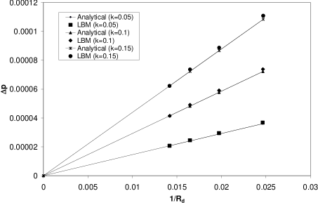
Figure 2: Pressure difference across axisymmetric drops as a function of radius for different values of the surface tension parameter $\kappa$; Comparison of computed results using the axisymmetric LBE model versus theoretical prediction based on the Laplace-Young relation. Quantities are in lattice units.

a maximum relative error of about $3\%$.

Another important test problem is that of an oscillating axisymmetric drop immersed in a gas. Since current versions of the LBE simulate a relatively viscous fluid, it is appropriate to compare the oscillation frequency with that of Miller and Scriven (1968) . In contrast to earlier analytical solutions on drop oscillations, this work considers viscous dissipation effects in the boundary layer at the interface. According to Miller and Scriven (1968), the frequency for the $n^{th}$ mode of oscillation for a drop is given by

$$\omega_{n}=\omega_{n}^{*}-\frac{1}{2}\alpha\omega_{n}^{*\frac{1}{2}}+\frac{1}{4}\alpha^{2},$$ (75)

where $\omega_{n}$ is the angular response frequency, and $\omega_{n}^{*}$ is Lamb’s natural resonance frequency expressed as Lamb (1932)

$$\left(\omega_{n}^{*}\right)^{2}=\frac{n(n+1)(n-1)(n+2)}{R_{d}^{3}\left[n\rho_{g}+(n+1)\rho_{l}\right]}\sigma.$$ (76)

$R_{d}$ is the equilibrium radius of the drop, $\sigma$ is the interfacial surface tension, and $\rho_{l}$ and $\rho_{g}$ are the densities of the two fluids. The parameter $\alpha$ is given by

$$\alpha=\frac{(2n+1)^{2}(\mu_{l}\mu_{g}\rho_{l}\rho_{g})^{\frac{1}{2}}}{2^{\frac{1}{2}}R_{d}\left[n\rho_{g}+(n+1)\rho_{l}\right]\left[(\mu_{l}\rho_{l})^{\frac{1}{2}}+(\mu_{g}\rho_{g})^{\frac{1}{2}}\right]},$$ (77)

where $\mu_{l}$ and $\mu_{g}$ are the dynamic viscosity of the two liquids. The subscripts $g$ and $l$ refer to the ambient gas and liquid phases, respectively. We consider the second mode of oscillation and analytical expressions for the time period are presented in Eq. (75).

The initial computational setup consists of a prolate spheroid of minimum ($R_{min}$) and maximum ($R_{max}$) radii of $40$ and $55$, respectively, placed in the center of the domain discretized by $201\times 101$ lattice sites. We consider the surface tension parameters: $\kappa=0.2$, and the density of the gas and the drop to be $\rho_{g}=0.1$ and $\rho_{l}=0.4$, respectively. The kinematic viscosity of both the gas and the drop are considered to be the same and given by $\nu_{g}=\nu_{l}=1.6667\times 10^{-2}$. Figure 3 shows the configurations of an oscillating drop at different times computed using the standard axisymmetric model with these conditions.

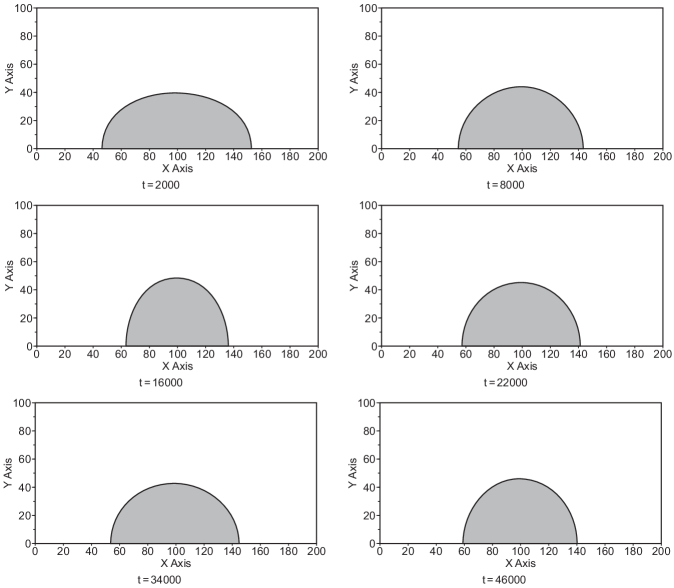
Figure 3: Configurations of an oscillating drop as a function of time; $R_{min}=40$, $R_{max}=55$, $\rho_{g}=0.1$, $\rho_{l}=0.4$, $\nu_{l}=\nu_{g}=1.6667\times 10^{-2}$. Quantities are in lattice units.

The drop changes from a prolate shape at $t=2000$ to oblate shape at $t=16000$. Such shape changes continue till the drop reaches its equilibrium spherical shape. Figure 4 shows the temporal evolution of the interface locations of the oscillating drop with the conditions above for two different surface tension parameter: $\kappa=0.02$ and $0.08$.

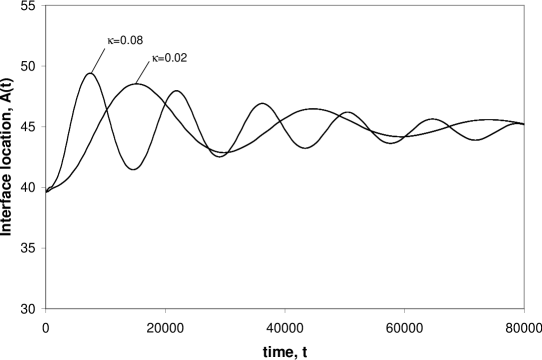
Figure 4: Interface location of an oscillating drop as a function of time for two values of the surface tension parameter $\kappa$; $R_{min}=40$, $R_{max}=55$, $\rho_{g}=0.1$, $\rho_{l}=0.4$, $\nu_{l}=\nu_{g}=1.6667\times 10^{-2}$. Quantities are in lattice units.

It is expected that increasing the surface tension will reduce the time period of oscillations. The computed ($T_{LBE}$) and analytical ($T_{anal}$) time periods, where $T_{anal}=2\pi/\omega_{2}$, when $\kappa=0.02$ are $29483$ and $29448$ respectively. As $\kappa$ is increased to $0.08$, $T_{LBE}$ and $T_{anal}$ become $14388$ and $14313$ respectively. It may be seen that the computed and analytical values agree well, the difference being less than $1\%$. Also, the time period decreases as $\kappa$ is increased, which is consistent with expectations.

Consider next the effect of changing the drop size on the time period of oscillations. Figure 5 shows the interface locations of an oscillating drop as a function of time for the following two initial sizes: $R_{min}=30$ and $R_{max}=45$; $R_{min}=40$, $R_{max}=55$. Reducing the drop size reduces its time period.

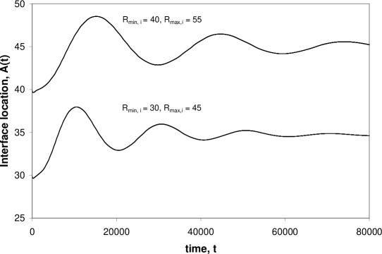
Figure 5: Interface location of an oscillating drop as a function of time for two drop sizes; $\rho_{g}=0.1$, $\rho_{l}=0.4$, $\nu_{l}=\nu_{g}=1.6667\times 10^{-2}$, $\kappa=0.02$. Quantities are in lattice units.

The computed time period of the larger drop is equal to $29483$, while that for the smaller drop is $20118$. Comparison of the computed time periods with the analytical solution shows that they agree within $1\%$ for these cases. Next, consider three different kinematic viscosities of the liquid: $\nu_{l}=1.6667\times 10^{-2},3.3333\times 10^{-2}$ and $5.0\times 10^{-2}$. Figure 6 shows the effect of drop viscosity on the temporal evolution of the interface locations of the drop.

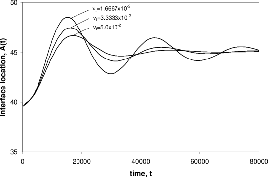
Figure 6: Interface location of an oscillating drop as a function of time for different kinematic viscosities $\nu_{l}$; $R_{min}=40$, $R_{max}=55$, $\rho_{g}=0.1$, $\rho_{l}=0.4$, $\kappa=0.02$. Quantities are in lattice units.

It is found that as the kinematic viscosity is increased the time period increases moderately which is consistent with the analytical solution. The computed time periods at these viscosities are $29483$, $31030$ and $32925$, while the analytical values are $29448$, $30597$ and $31318$, respectively, with a maximum error within $5.1\%$.

The third test problem considered here is that of the break-up of a cylindrical liquid column into drops, a fascinating problem of long standing theoretical and practical interest. In a seminal work, Rayleigh (1878)  showed through a linear stability analysis of an inviscid column of cylindrical liquid of radius $R_{c}$ that the column will be unstable if the axisymmetric wavelength of any disturbance $\lambda_{d}$ is longer than its circumference, i.e. the wave number $k^{*}=2\pi R_{c}/\lambda_{d}$ should be less than one. Later, the theoretical analysis was extended to more realistic conditions by including viscosity. In the last three decades, several experimental and numerical investigations have also been performed. To evaluate the axisymmetric LBE model, we study the Rayleigh capillary instability for different wavenumbers. Initial studies carried out with $k^{*}>1$ showed that the liquid does not break-up. We will now present results of cases with break-up. Consider a cylindrical liquid column of radius $R_{c}=45$ subject to an axisymmetric co-sinusoidal wavelength $\lambda_{d}=320$, i.e. $k^{*}=0.88$. To simulate the dynamics of instability for this wavenumber, we consider a domain discretized by $321\times 151$ lattice sites with $\rho_{g}=0.1$, $\rho_{l}=0.4$, $\nu_{g}=\nu_{l}=6.6667\times 10^{-2}$ and $\kappa=0.1$. Since $k^{*}<1$, it is expected that the liquid column would eventually breakup. Figure 7 shows the configurations of the liquid column at different times. As time progresses, the imposed interfacial disturbances on the

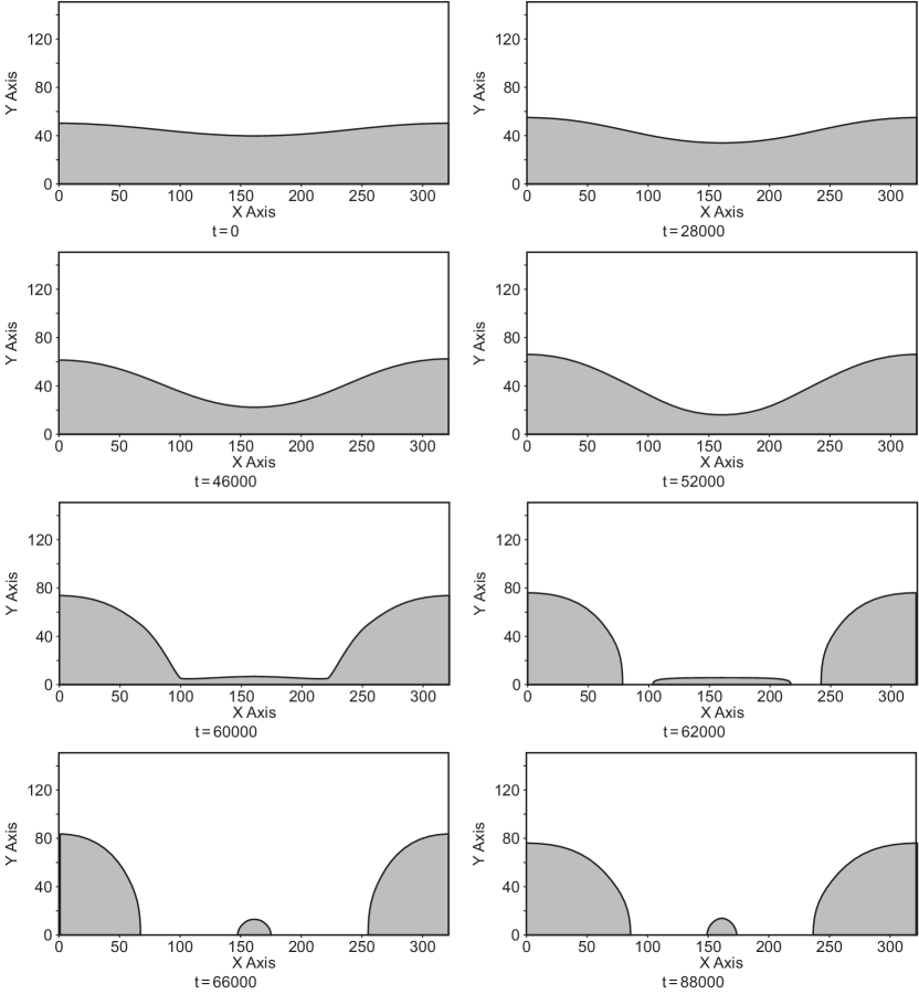
Figure 7: Configurations of a cylindrical liquid column at different times undergoing Rayleigh breakup and satellite droplet formation; $k^{*}=0.88$, $\rho_{g}=0.1$, $\rho_{l}=0.4$, $\nu_{l}=\nu_{g}=6.6667\times 10^{-2}$. Quantities are in lattice units.

liquid column grow. At $t=28000,46000$ $52000$, the cross-section of the column becomes progressively thinner in the center, and by mass conservation, the ends becomes larger. At $t=60000$, notice that a bead-type structure is formed at the ends and with a thin ligament between them. Such a structure has been observed in experiments Eggers (1997) and in other numerical simulations Ashgriz and Mashayek (1995). Eventually, the column breaks up forming a thin ligament in the middle, which then becomes a satellite droplet.

Let us now increase the wavelength of the disturbance to $\lambda_{d}=600$, keeping the physical parameters the same as before. We consider a domain represented by $601\times 151$ lattice sites. Since, $R_{c}=45$ as before, the wavenumber is $0.47$. Figure 8 shows the temporal evolution of the configurations of the liquid column at this reduced wavenumber. The axisymmetric disturbance grows with time.

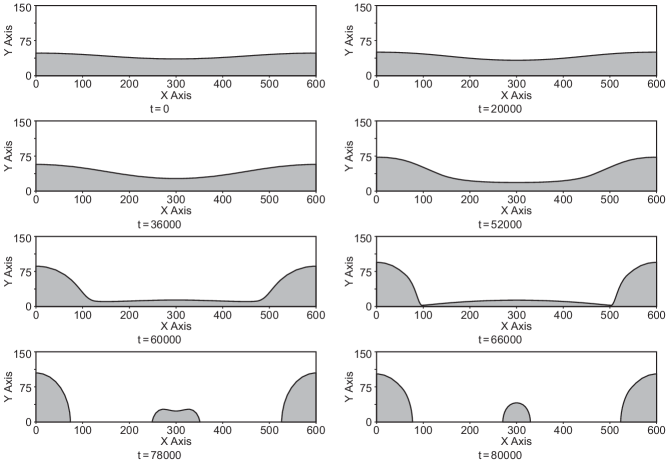
Figure 8: Configurations of a cylindrical liquid column at different times undergoing Rayleigh breakup and satellite droplet formation; $k^{*}=0.47$, $\rho_{g}=0.1$, $\rho_{l}=0.4$, $\nu_{l}=\nu_{g}=6.6667\times 10^{-2}$. Quantities are in lattice units.

Since the wavelength is longer, it can be noticed that the ligament that is formed during the Rayleigh instability is also longer. As a result, after the column breaks up, a larger satellite droplet is formed. To express the drop size distribution with wave numbers more quantitatively, we plot the non-dimensional size of the main and satellite drops, $r^{*}=R/R_{c}$, as a function of wave number, $k^{*}$ in Fig. 9. It may be noted that Rayleigh’s

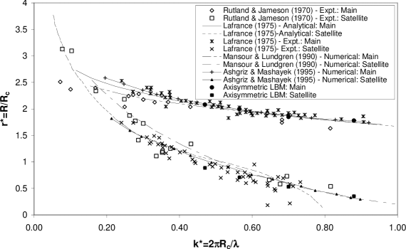
Figure 9: Drop sizes resulting from Rayleigh breakup of liquid cylindrical column as a function of wave number $k^{*}$. Quantities are dimensionless.

original analysis predicts only the onset of breakup and not the formation of satellite droplets. To predict analytically satellite droplet formation, it has been shown that at least a third-order perturbation analysis of the Navier-Stokes equations (NSE) is needed Lafrance (1975). Computations based on direct solutions of the NSE also predict the formation of the satellite droplets.

To evaluate the drop size distribution computed using the axisymmetric LBE model, we consider the experimental data of Rutland and Jameson (1971),  the experimental data and analytical solution based on a third-order perturbation analysis of the NSE by Lafrance (1975),  a boundary integral solution of the NSE by Mansour and Lundgren (1990)  and a finite element solution of the NSE by Ashgriz and Mashayek (1995).  It can be seen in the figure that as long as the wavenumber is less than one, as expected there will be a satellite droplet formation. As the wavenumber is reduced, the sizes of both the main drop and satellite droplet increases. The rate of increase of the size of the satellite droplet is greater than that of the main drop. Notice that there is considerable scatter in the available data in the figure. The computed results from the axisymmetric LBE model are presented for wavenumbers greater than or equal to $0.47$. Ignoring the two experimental data points of Lafrance (1975) for the satellite drop sizes that deviate considerably from the others, we find that the axisymmetric model is able to reproduce the drop size distribution quantitatively within $12\%$.

The axisymmetric model has been employed to study head-on collisions of drops of radii $R_{1}$ and $R_{2}$ approaching each other with a relative velocity $U$. The dynamics and outcome of colliding drops is characterized mainly by the Weber number, $We$ defined by $We=\rho_{l}(R_{1}+R_{2})U^{2}/\sigma$ Qian and Law (1997). Additional parameters that may have an influence are the Ohnesorge number, $Oh$, defined by $Oh=16\mu_{l}/\sqrt{\rho_{l}R_{1}\sigma}$ and ratios of liquid and gas densities($r$) and dynamic viscosities ($\lambda$). According to experiments Qian and Law (1997), it is expected that lower $We$ collisions lead to coalescence while higher $We$ to separation by reflexive action. Figures 10 and 11 present drop configurations at $We=20$ and $We=100$ respectively. Notice that at $We=20$, the drops coalesce, while at $We=100$, they eventually separate

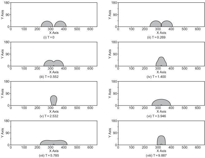
Figure 10: Colliding drops at different times $T$; $We=20$, $Oh=0.589$, $r=4$, $\lambda=1$. Time is normalized by the relative velocity between the drops and their diameter. Axes are in lattice units.

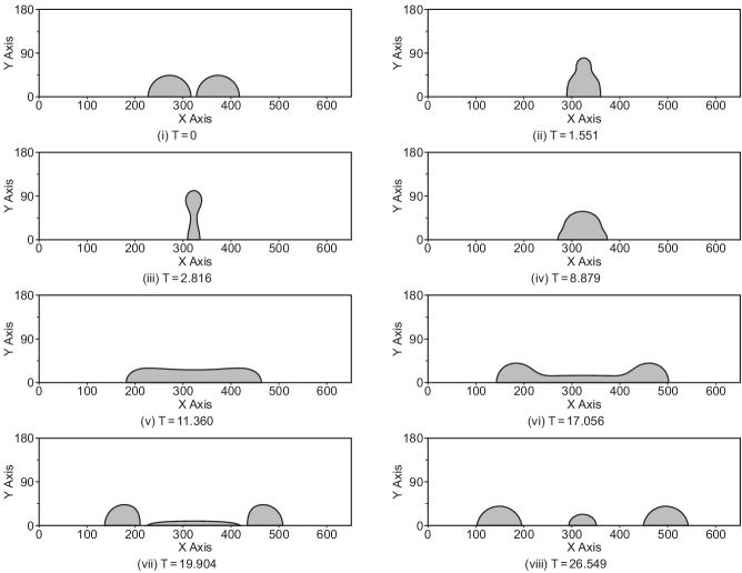
Figure 11: Colliding drops at different times $T$; $We=100$, $Oh=0.589$, $r=4$, $\lambda=1$. Time is normalized by the relative velocity between the drops and their diameter. Axes are in lattice units.

with the formation of a satellite droplet, which are consistent with experimental observations. Also notice that for the latter case, the temporarily coalesced drop undergoes various stages of deformation which are consistent with a recent theoretical analysis Roisman (2004). Additional details of these and other studies of drop collisions are given in Ref. Premnath and Abraham (2004b).

V Summary

In this paper, a LB model for axisymmetric multiphase flows is developed. The axisymmetric model is developed by adding source terms to the standard Cartesian BGK LBE. The source terms, which are temporally and spatially dependent, represent the axisymmetric contributions of the order parameter, which distinguish the different phases, as well as inertial, viscous and surface tension forces. Consistency of the model in achieving the desired axisymmetric flow multiphase behavior is established through the Chapman-Enskog multiscale analysis. The analysis shows that the axisymmetric macroscopic conservation equations are recovered in the continuum limit. An axisymmetric model with reduced compressibility effects is then developed to improve its computational stability. In this version, a transformation is introduced to the distribution function in the LBE such that it reduces the compressibility effects. Comparisons of computed axisymmetric equilibrium drop formation and oscillations, Rayleigh capillary instability, breakup and formation of satellite drops liquid cylindrical liquid columns and the outcomes of head-on drop collisions with available data show satisfactory agreement. The maximum error for the frequency of drop oscillations is less than $5.1\%$ and that for drop sizes as a result of Rayleigh breakup is $12\%$.