Conditional Probability as a Measure of Volatility Clustering in Financial Time Series

Abstract

In the past few decades considerable effort has been expended in characterizing and modeling financial time series. A number of stylized facts have been identified, and volatility clustering or the tendency toward persistence has emerged as the central feature. In this paper we propose an appropriately defined conditional probability as a new measure of volatility clustering. We test this measure by applying it to different stock market data, and we uncover a rich temporal structure in volatility fluctuations described very well by a scaling relation. The scale factor used in the scaling provides a direct measure of volatility clustering; such a measure may be used for developing techniques for option pricing, risk management, and economic forecasting. In addition, we present a stochastic volatility model that can display many of the salient features exhibited by volatilities of empirical financial time series, including the behavior of conditional probabilities that we have deduced.

PACS numbers: 89.65.Gh, 89.75.Da, 02.50.Ey

I Introduction

Forecasting from time series data necessarily involves an attempt to understand uncertainty; volatility or the standard deviation is a key measure of this uncertainty and is found to be time-varying in most financial time series. The seminal work of Engle Engle , that first treated volatility as a process rather than just a number to estimate, led to tremendous efforts in devising dynamical volatility models in the last two decades. These are of great importance in a variety of financial transactions including option pricing, portfolio and risk management. Excess volatility (well beyond what can be described by a simple Gaussian process) and the associated phenomenon of clustering benoit ; Fama are believed to be the key factors underlying many empirical statistical properties of asset prices, characterized by a few key “stylized facts” intro1 ; intro2 ; intro3 ; intro4 described later. A good measure of volatility clustering (roughly speaking, large and small changes in asset prices are often followed by large and small changes respectively) is thus important for understanding financial time series and for constructing and validating a good volatility model. The most popular characterization of volatility clustering is the correlation function of the instantaneous volatilities evaluated at two different times, which shows persistence up to a time scale of more than a month. It has also been established that there is link between asset price volatility clustering and persistence in trading activity (for an extended empirical study on this, see Ref. Plerou ). However, the underlying market mechanism for volatility clustering is not clear. The aim of our paper is not to elucidate the mechanism for volatility clustering, but to introduce a more direct measure of it. Specifically, we propose that the conditional probability distribution of asset returns $r$ over a period $T$ (given the return, $r_{p}$, in the previous time period )can be fruitfully used to characterize clustering. This is a direct measure based on return over a time lag instead of instantaneous volatility and we believe is more relevant to volatility forecasting. We analyze stock market data using this measure, and we and have found that the conditional probability can be well described by a scaling relation: $P(r|r_{p})=\frac{1}{w(r_{p})}f(r/w(r_{p}))$. This scaling relation characterizes both fat tails and volatility clustering exhibited by financial time series. The fat tails are described by a universal scaling function $f(z)$. The functional form of the scaling factor $w(r_{p})$, on the other hand, contains the essential information about volatility clustering on the time scale under consideration. The scaling factors we obtain from the stock market data allow us to identify regimes of high and low volatility clustering. We also present a simple phenomenological model which captures some of the key empirical features.

The key “stylized facts” about asset returns include the following: The unconditional distribution of returns shows a scaling form (fat tail). The distribution of returns $r$ in a given time interval (defined as the change in the logarithm of the price normalized by a time-averaged volatility) is found to be a power law $P(|r|>x)\sim x^{-\eta_{r}}$ with the exponent $\eta_{r}\sim 3$ for U.S. stock marketsgopikrishnan ; gabaix , well outside the Lévy stable range of 0 to 2. This functional form holds for a range of intervals from minutes to several days while for larger times the distribution of the returns is consistent with a slow crossover to a normal distribution. Another key fact is the existence of volatility clustering in financial time series that is by now well established benoit ; Fama ; Engle ; Bollerslev ; intro4 ; it can be seen, for example, in the absolute value of the return $|r|$, which shows positive serial correlation over long lags (the Taylor effect Taylor ). This long memory in the autocorrelation in absolute returns, on a time scale of more than a month, stands in contrast to the short-time correlations of asset returns themselves. Fat tails have been the subject of intense investigation theoretically from Mandelbrot’s pioneering early workbenoit using stable distributions to agent-based models of Bak et al.bak and Luxlux0 ; lux (See Ref. LeBaron for a survey of research on agent based models used in finance). The key problem is to elucidate the nature of the underlying stochastic process that gives rise to both volatility clustering and the power-law (fat) tails in the distribution of asset returns.

II Conditional Probability and Scaling Form

In an effort to seek a direct quantitative characterization of clustering we consider $P(r|r_{p})$, the probability of the return $r$ in a time interval of duration $T$, conditional on the absolute value of the return $r_{p}$ in the previous interval of the same duration. (We emphasize that the probability is not conditioned on the value of the return at an instant.) By varying $T$, we can check volatility clustering on different time scales. There is a growing literature on conditional measures of distribution for analyzing financial time series (for a review, see Ref. Malevergne and references therein). For example, the conditional probability of return intervals has been used recently to study scaling and memory effects in stock and currency data Yamasaki .

We have analyzed both the high frequency data and daily closing data of stock indices and individual stock prices using the conditional probability as a probe. Here we only present results of our analysis of high frequency data of QQQ (a stock which tracks the NASDAQ 100 index) from 1999 to 2004 and daily closing data of the Dow Jones Industrial Average from 1900 to 2004. We emphasize that the properties of the financial time series we present are rather general: we have checked that the same properties are also exhibited in other stock indices and future data (for example, the Hang Seng Index, Russell 2000 Index, and German government bond futures) as well as individual stocks. We have checked, as was found in the previous studies gopikrishnan , that the probability distribution of the returns in the time intervals $T=1,2,4,8,16,32$ days for DJIA exhibits a fat power-law tail with an exponent close to $-4$; this appears to be true for most stock indices and individual stock data.

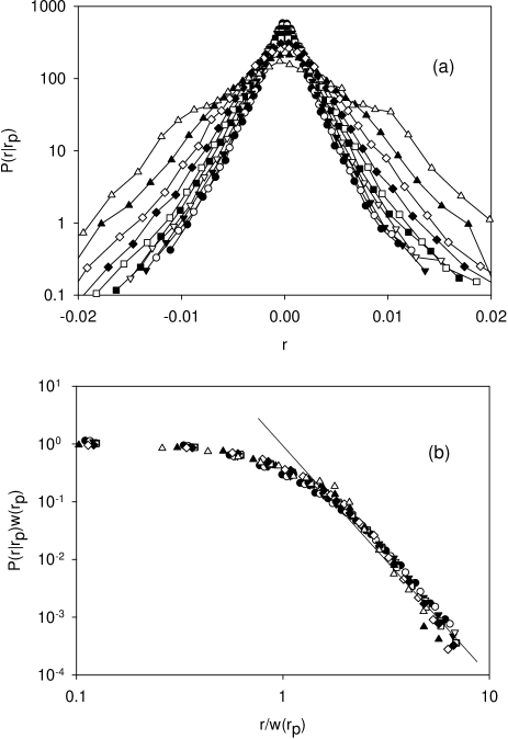
Figure 1: (a) Conditional probability of return for $T=5$ minutes in QQQ. Different curves correspond to 10 different absolute values of the return $r_{p}$ in the previous interval, which are groups of bins centered at values ranging from $8.4\times 10^{-4}$ to $0.011$. The larger the value of $r_{p}$, the large the width of the distribution. (b) The conditional probability distribution of return of QQQ (shown in (a)), when scaled by a scale factor $w(r_{p})$, collapses to a universal curve. $r_{p}$ is the absolute value of the return in the previous interval. The tail of the probability distribution can be described by a power law with the exponent approximately equal to $-4$.

We calculate $P(r|r_{p})$, by grouping the data into different bins according to the value of $r_{p}$. In Figure 1(a) we display $P(r,T|r_{p},T)$ for $T=5$ minutes for different values of $r_{p}$. It is clear from the figure that there is a positive correlation between the width of $P(r|r_{p})$ and $r_{p}$. What is more interesting is that, when $r$ is scaled by the width of the distribution (the standard deviation of the conditional return), $w(r_{p})$, the different curves of conditional probability collapse to a universal curve: $P(r|r_{p})=w(r_{p})^{-1}\bar{P}(r/w(r_{p}))$. Evidence for this is displayed in Fig. 1(b). Note that on the time scales we have analyzed, the probability distribution is symmetric with respect to $r$. Consequently, in Fig. 1(b) we have only displayed the absolute value of the return. The data collapse is good for a wide range of $T$, and the curves display a power-law tail with a well-defined exponent of approximately $-4$.

We examine next the behavior of the scale factor $w(r_{p})$ on $r_{p}$. Fig. 2 shows a plot of the scale factor $w(r_{p})$ vs. $r_{p}$ for different values of $T$. It can be seen from the figure that there is a crossover value $r_{c}(T)$: for $r_{p}<r_{c}(T)$, $w$ is almost constant, while for $r>r_{c}(T)$, $w$ increases with $r_{p}$. The degree of the dependence of $w$ on $r_{p}$ can be taken as an indication of strength of volatility clustering. If there is no volatility clustering $w$ will not depend on $r_{p}$. Note that there is a strong clustering at small $T$. As $T$ increases, the strength of clustering gradually decreases, indicating a crossover to the non-clustering regime. As $T$ increases beyond the time scale of volatility clustering, the clustering disappears. This crossover can not be seen in the QQQ data as the time scales involved are small. Our analysis of DJIA data show an indication of such crossover at the time scale of a few months. In this paper, we do not separate the cases of positive and negative returns in the previous time interval. Thus we do not show explicitly the well-known leverage effect, first expounded by Black Black . We have checked that the scaling and data collapse we obtained are equally valid when we separate out the cases of positive and negative returns in the previous interval. The leverage effect is reflected in the scaling factor $w(r_{p})$, which shows $w(-r_{p})>w(r_{p})$ for $r_{p}>0$ in the real data.

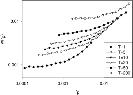
Figure 2: The scale factor $w(r_{p},T)$ vs $r_{p}$ (the absolute value of the return in the previous interval) for different values of $T$, arising from analysis of QQQ data. The dependence is seen to be almost linear for sufficiently large $r_{p}$

Figure 3 shows that the same scaling form is also exhibited in DJIA data. We have checked that the data collapse extends also to data for different values of $T$ in addition to different values of $r_{p}$ displayed here.

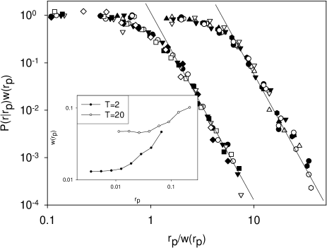
Figure 3: Conditional probability of return for $T=2$ and $T=20$ days in DJIA data. The data corresponding to $T=20$ have been shifted to the right for easy viewing. Different curves correspond to 8 different absolute values of the return $r_{p}$ in the previous interval. The inset shows the dependence of the width $w(r_{p})$ on $r_{p}$. The tail of the probability distribution can be described by a power law with the exponent approximately equal to $-4$.

The data collapse we have displayed for different $r_{p}$ and different $T$, the power-law behavior including the value of the exponent, and the behavior of the scale factor which encapsulates features of volatility clustering are the same across data from several other stock indices listed earlier and individual stocks. This empirical universality can be stated as

$$P(r|r_{p})=\frac{1}{w(r_{p},T)}f(r/w(r_{p},T)).$$ (1)

Here $f(z)$ is a universal function describing the universal fat tail in the distribution. $f(z)$ satisfies $f(z)\rightarrow$ constant as $z\rightarrow 0$, $f(z)\rightarrow 1/z^{4}$ as $z\gg 1$, and $\int^{\infty}_{0}f(z)dz=1$. The dependence of $w(r_{p},T)$ on $r_{p}$, on the other hand, describes the volatility clustering at the time scale $T$. If $w(r_{p})$ is a constant (independent of $r_{p}$), then $P(r|r_{p})$ does not depend on $r_{p}$, and there is no volatility correlation or clustering. The conditional probability distribution contains information about the conditional average of the moments $<r^{q}>_{r_{p}}$ of the distribution as well as various volatility correlation functions such as $<r^{2}r_{p}^{2}>$. Given the scaling form we can evaluate these averages and correlation functions in terms of $w(r_{p})$, which is itself given by $w(r_{p})=\sqrt{<r^{2}>_{r_{p}}}$. In particular, we have the moments of the conditional probability distribution given by $M_{q}(r_{p})=<r^{q}>_{r_{p}}=C_{q}w^{q}(r_{p})$ ($C_{q}$ is a universal constant) and $<r_{p}^{2}r^{2}>=\int dr_{p}Q(r_{p})w^{2}(r_{p})r^{2}_{p}$, where $Q(r)$ is the unconditional probability distribution of the return. We believe that this scaling form provides a new and rather complete measure of volatility clustering.

III Model and Discussion

In the following we will provide the outline of a model that captures the key features exhibited in the conditional probability distribution of stock market data. In a stochastic volatility model, the one-step asset return at time $t$ is written as $\Delta_{t}=\delta_{t}z_{t}$, where $z_{t}$ is a Gaussian random variable with zero mean and unit variance and $\delta_{t}$ is magnitude of the price change. For the relatively short time scales we are interested in we have set the intrinsic growth rate to zero. The distribution of $r$ depends on the dynamics of $\delta_{t}$: Slow changes in $\delta_{i}$ lead to volatility clustering.

There exist a few classes of volatility models that have been used to describe the dynamics of $\delta_{t}$. These include the widely used models based on GARCH-like processes Engle , and more recently, the models based on a multifractal random walk (MRW) MRW that will be discussed later. In our model, the dynamics of $\delta(t)$ is specified via the random variable $n(t)$, with $\delta(t)=\delta_{0}\gamma^{n(t)}$. In order to describe both the behavior of probability distributions and temporal correlations we have devised the following model for the evolution of $n(t)$. The time evolution of the variable $n$ is assumed to be independent of the change in $S(t)$ and $n(t)$ executes a random walk with reflecting boundaries: We enforce the condition $n(t)\geq 0$; thus $\delta_{0}$ is the minimum value of $\delta(t)$. An upper bound in $n$, $n_{max}$, can also be incorporated without affecting the scaling behavior of the model. We typically choose $\gamma^{n_{max}}\sim 30$. The change in $n(t)$, $\delta n(t)$ is given by

$$\delta n(t)\, = \,\eta_{t}\,+\,\alpha\{\sum_{i=1}^{N_{c}}[K(i+1)-K(i)]\eta_{t-i}+K(1)\eta_{t}$$ (2)

$$-K(N_{c}+1)\eta_{t-N_{c}}\}\,-\,\beta\overline{\eta}\,.$$

In the preceding $\{\eta_{j}\}$ are independent random variables that assume the value $+1$ with probability $p$ and $-1$ with probability $1-p$. This asymmetry builds in the tendency to decrease the volatility. The mean value of $\eta_{i}$, $2p-1<0$ is denoted by $\overline{\eta}$. We comment on the implications of the different terms next.

We focus on the limit $\alpha=0$ and $\beta=0$ first since it is amenable to analytic investigation; this model is related to a model discussed in Ref. chen . Note that this limit already builds in volatility clustering as it takes many steps to change $n(t)$ significantly. It is easy to show that, the steady-state probability distribution of $n$ is given by $P(n)=(1-e^{-\lambda})e^{-\lambda n}\sim\lambda e^{-\lambda n}$, where $\lambda=\ln((1-p)/p)$. The distribution of $\delta(t)$ is then given by a power-law, $P(\delta)\sim\delta^{-\lambda/\ln\gamma-1}$. This mechanism for generating a power-law distribution was first noted by Herbert Simon simon in 1955. We have studied this limiting case of the model numerically and find that many features of the conditional probability distribution exhibited by the real data including the power law and scaling behaviors are reproduced. We can show analytically that the conditional probability distribution exhibits scaling collapse, and that scale-invariant behavior with a power law tail (with the exponent $-4$ if we choose $p=1/(1+\gamma^{2})$) exists for $r>\sigma_{c}$, where $\sigma_{c}=\sigma_{0}\gamma^{(T/\delta t)(1-2p)}$. The numerical data in fact show a somewhat larger range of power-law behavior. The re-scaling factor required for data collapse is simply proportional to $r_{p}$ from our analysis, as we have observed from the real data and from numerical simulations of model when $r_{p}$ is not too small. The simple limit captures important features of volatility clustering reflected in conditional probability distributions.

The second term in Eq. (2) is based on the multifractal random walk model that builds in long-time correlations via a logarithmic decay of the log volatility correlation $\langle\log|r(t+\tau)|\log|r(t)|\rangle$. This term allows us to reproduce the more subtle temporal autocorrelation behavior observed in the data and follows the implementation in Ref. Sornette . The long-term memory effects are incorporated by making the change in $n(t)$ depend on the steps $\eta_{t-i}$ at earlier times with a kernel given by $K(i)\,=\,1/\sqrt{i}$ (this corresponds to the MRW part of the model given by $n(t)=\alpha\sum_{i=1}^{N_{c}}K(i)\eta_{t-i}$) and allowing memory up to $N_{c}$ time steps, chosen to be $1000$ in our simulations. The final term allows us to control the rate of drift to lower values of $n$. We have simulated this model with $\alpha_{0}=0.1$ ($\alpha=\alpha_{0}/\ln(\gamma)$) and $\beta\approx 1.3$ for $\gamma=1.05$ and displayed the results for $P(r|r_{p})$ in Figure 4. The model with the stated parameters reproduces the fat tail in the unconditional probability distribution for $r$ observed in the data. The non-universal scale factor $w(r_{p})$ is similar to those found from our empirical analysis. We have also checked that this model retains the same temporal behavior in the log-volatility correlation exhibited by the pure MRW model. Thus the model we have investigated is capable of reproducing both probability distributions (conditional and unconditional) and temporal autocorrelations. We note in passing that the model as it stands cannot be used to study the leverage effect; however, it can be modified to do so.

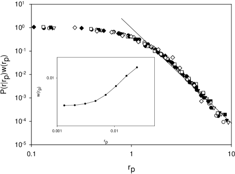
Figure 4: The scaled conditional probability distributions of return for the mixed model given by Eq. (2) with $\gamma=1.05$, $\alpha_{0}=0.1$, and $\beta=1.3$. The time lag is $T=10$. The curves, corresponding to different absolute values of the return $r_{p}$ in the previous interval collapse on to a universal curve when scaled by a scale factor $w(r_{p})$. The tail of the probability distribution is again described by a power law with the exponent equal to $-4$. The inset shows the dependence of $w(r_{p})$ on $r_{p}$.

In summary, we have proposed a direct measure of volatility clustering in financial time series based on the conditional probability distribution of asset returns over a time period given the return over the previous time period. We discovered that the conditional probability of stock market data can be well described by a scaling relation, which reflects both fat tails and volatility clustering of the financial time series. In particular, the strength of volatility clustering is reflected in the functional form of the scaling factor $w(r_{p})$. By extracting $w(r_{p})$ from market data, we are able to estimate the future volatility over a time period, given the return in the previous period. This may be useful in modelling financial transactions including option pricing, portfolio and risk management; all these depend crucially on volatility estimation. The clustering of activities and fat tails in the associated distribution are very common in the dynamics of many social Barabasi and natural phenomena (e.g. earthquake clustering Kagan ). The conditional probability measure we have presented in this paper may serve as a useful tool for characterizing other clustering phenomena.

This work was supported by the National University of Singapore research grant R-151-000-032-112.

References

- (1) R. F. Engle, Econometrica 50, 987 (1982).
- (2) B. Mandelbrot, J. Business 36, 394 (1963).
- (3) E. F. Fama, J. Business 38, 34 (1965).
- (4) R. Mantegna and H. E. Stanley An introduction to econophysics (Cambridge University Press, Cambridge, 1999).
- (5) J.-P. Bouchaud and M. Potters Theory of financial risks: from statistical physics to risk management (Cambridge University Press, Cambridge, 2000).
- (6) R. Cont Quantitative Finance 1, 223 (2001).
- (7) R. F. Engle and A. J. Patton Quantitative Finance 1 237 (2001).
- (8) V. Plerou, P. Gopikrishnan, L.A.N. Amaral, X. Gabaix, and H.E. Stanley, Phys. Rev. E 62, R3023 (2000).
- (9) P. Gopikrishnan, M. Meyer, L. A. N. Amaral, and H. E. Stanley, Euro. Phys. J. B 3, 139 (1998).
- (10) X. Gabaix, P. Gopikrishnan, V. Plerou, and H. E. Stanley, Nature 423, 267 (2003).
- (11) T. Bollerslev, Journal of Econometrics 31, 307 (1986).
- (12) S. Taylor, Modelling the financial time series (John Wiley, New York 1986).
- (13) P. Bak, M. Paczuski, and M. Shubik, Physica A 246, 430 (1997).
- (14) T. Lux and M. Marchesi, Nature 397, 498 (1999).
- (15) T. Lux, Journal of Economic Behavior and Organization 33, 143 (1998).
- (16) H. Simon, Biometrika 42, 425 (1955).
- (17) B. LeBaron, in Handbook of Computational Economics, Vol. 2: Agent-Based Computational Economics, eds. L. Tesfatsion & K.L. Judd (North-Holland, Amsterdam), Chapter 9 (2006).
- (18) Y. Malevergne and D. Sornette Extreme Financial Risks (from dependence to risk management) (Springer, Heidelberg 2005).
- (19) F. Black, Proc. Bus. Econ. Statist. Sect. Am. Statist. Assoc., 177 (1976).
- (20) E. Bacry, J. Delour, and J. F. Muzy, Phys. Rev. E 64, 026103 (2001).
- (21) D. Sornette, Y. Malevergne, J. F. Muzy, Risk Magazine 16(2), 67 (2003).
- (22) K. Yamasaki, L. Muchnik, S. Havlin, A. Bunde, and H. E. Stanley, Proc. Natl. Acad. Sci. USA 102, 9424 (2005).
- (23) K. Chen and C. Jayaprakash, Physica A 324, 258 (2003).
- (24) A.-L. Barabasi, Nature 435, 207 (2005).
- (25) Y. Y. Kagan and D. D. Jackson, Geophys. J. Int. 104, 117 (1991).