Describing two-dimensional vortical flows :
the typhoon case

Abstract

We present results of a numerical study of the differential equation governing the stationary states of the two-dimensional planetary atmosphere and magnetized plasma (within the Charney Hasegawa Mima model). The most strinking result is that the equation appears to be able to reproduce the main features of the flow structure of a typhoon.

1 Introduction

There is a well known similarity between the two-dimensional models of the planetary atmosphere and the magnetized plasma. In the absence of dissipation the models can be reduced to differential equations having the same structure: the Charney equation for the nonlinear Rossby waves , in the physics of the atmosphere [1]; and the Hasegawa-Mima equation for drift wave turbulence, in plasma physics [2]. They are similar with the Navier-Stokes equation because they have two conserved quantities, the energy and the enstrophy. This in principle allows states of negative temperatures, or, equivalently, these models support a trend to organised vortical flow. It results the possibility to have as solutions coherent structures (vortices) besides the turbulent states characterised by spectral cascade.

These analytical models have led to a serious advancement of our knowledge in both fields. However the stationary states appear to be described within these models by a reduced equation having a too wide generality, representing actually something as a constraint with weak ability to identify unequivocally the real solutions: it simply states that at stationarity the advection of the vorticity by the velocity vector field vanishes. In reality, numerical simulations show that the stationary states reached in relaxation are very regular and persist for a long time period and that this set of asymptotic states is not the huge space of functions able to fulfill the constrained mentioned above. The fluid evolves at relaxation toward a reduced subset of functions, characterized by regular shape of the streamfunction [12], [13], [14], [15] (and references therein). At the oposite limit the turbulent regime can be treated with renormalization group methods [16].

It is well-known that the same phenomenon exists in the case of the ideal fluid described by the Euler equation. By experiments and numerical simulation it has been shown that the ideal fluid evolves at relaxation toward a very ordered flow pattern, consisting of two (positive and negative) vortices and that this state persists for very long times, being limitted by only the effect of some residual dissipation. From numerical simulations it has also been inferred the form of the flow function. It has been found that the streamfunction obeys, in these states, the sinh-Poisson equation. Montgomery and his collaborators have developed a theoretical statistical model which explains the appearence of this equation in this context [3], [4], [5], [6], [7], [8], [9]. Later, the equation has also been derived by formulating the continuum version of point-like vortices as a field theoretical model of interacting gauge and matter fields in the adjoint representation of $SU\left(2\right)$ [17]. The essential point of the latter derivation was the self-duality of the relaxation states of the fluid.

No equation (similar to the sinh-Poisson equation in the Euler fluid case) has been found for the Charney-Hasegawa-Mima (CHM) equation, despite a considerable effort [10], [11]. However, as mentioned before, there are convincing experimental and numerical indications that the fluids (atmosphere and plasma) evolve to a reduced subset of states.

We have developed a field theoretical model for the point-like vortices with short range interaction, based on Chern-Simons action for the gauge field in interaction with the nonlinear matter field, again in $SU\left(2\right)$ algebra. It is then possible to derive the energy as a functional that becomes extremum on a subset of stationary states and presents particular properties. The general characterization of this family of states is their self-duality, which here means that the energy functional becomes minimum because the square terms are all vanishing, leaving as lower bound a quantity with topological meaning. A very detailed account of the derivation is in Refs. [18], [19].

The result is a set of equations parametrized by the solutions of the Laplacean equation in two-dimensions.

The simplest of these equations is

$$\Delta\psi+\frac{1}{2p^{2}}\sinh\psi\left(\cosh\psi-p\right)=0$$ (1)

(where $p$ is a positive constant). There are already some confirmations that this is the equation governing the asymptotic stationary states of the CHM fluids : the scatterplots of $\left(\psi,\omega\right)$ = (streamfunction, vorticity) obtained in experiments [20] and the scatterplots obtained in numerical simulations [10] are very similar to the nonlinear term of Eq.(1).

The objective of this work is to provide the first elements resulting from a numerical investigation of this equation.

The results are summarised here. This differential equation is able to reproduce the main two-dimensional features of the typhoon vortical flow. In the physics of the atmosphere, it seems that other examples, like the tropical cyclones, can be reproduced by solutions of this equation. The following are the features we consider as very particular to the typhoon morphology (in $2D$)  [21], [22], [23], [24]:

1. The very narrow dip of the azimuthal velocity (mean tangential wind) in the center of the vortex, compared with the very large extension in space. This is characterized by the “radius of the maximum tangential wind” and this radius, as mentioned, is much smaller than the diameter of the vortex. Our equation is able to generate solutions with this structure.

2. The slow decay of the magnitude of the azimuthal velocity toward the periphery, compared with the very fast decay toward the center; this is reproduced by the solutions of this equation.

3. The very low magnitude (almost vanishing) of the vorticity over most of the vortex (approx. from the radius of maximum wind to the periphery), while the magnitude in a narrow central region is extremely high. This feature is also reproduced by the equation.

4. quantitatively, we obtain for the diameter of the typhoon’s eye a relatively good magnitude. The vorticity is higher than in observations but not far from the realistic range.

We have very encouraging results of studies on plasma vortices, but they are not reported here. In plasma physics, the symmetrical, stable, vortical structures observed in experiments in the linear machine seem to belong to the class of solutions of this equation. We have also obtained several solutions that are very similar to the crystals of vortices, known from experiments.

2 Numerical studies of the equation

The numerical solution of this equation appears to be very difficult. This may be explained by the fact that the exponentials of the two functions $\sinh$ and $\cosh$ are very rapidly-varying functions and any perturbation is amplified and propagated in the solution.

In addition, the Laplace operator has spurious solutions with exponential behavior that have to be eliminated by the numerical procedure.

The paper of McDonald [25] on the numerical integration of the sinh-Poisson equation is very helpful in understanding the problems related to a numerical treatment of our equation. However the approach proposed in that paper requires to use a small mesh, specifically for excluding the spurious modes of the Laplacean. In the case of our equation, the vortices require a reasonable detailed description and this needs larger meshes. Then the problem of the precision of integration procedure arises and, if the initialization happens to be far from one of the solution, the number of iteration of the solver is high and the errors accumulate, leading to lack of convergence. It may be supposed that the solutions would be similar to those of the sinh-Poisson equation, but structures with sharp spatial variation may be possible [26].

The structure of the function space representing the union of attractors for the various solutions of this equation appears to be very complex. This immediately translates into serious obstacles in the attempt to reach one of the presumed solution. The main instrument is, naturally, the initialization, i.e. to start the integration in the right subspace, representing the attractor of that solution. Since there is no available analytical description of this space, the search is simply a problem of guessing a reasonable initial function and to repeat as many times as necessary. One of the specific behaviors is the tendency of driving the solution toward the constant value

$$\psi=\psi_{b}^{\left(1,2\right)}$$ (2)

(see Eq.(2.2)) which trivially verifies the equation. This seems to imply that there is a large attractor in the function space around these constant solutions. The solution which is larger in absolute magnitude is less stable since any fluctuation around the constant generates high vorticity. We underline that the integrations described here are not radial (i.e. unidimensional).

With all the difficulties of getting a right initial positioning in the integration procedure we note however that the solution with the typhoon morphology appears instistently from a wider class of initial shapes.

2.1 The numerical code

We use the code “GIANT A software package for the numerical solution of very large systems of highly nonlinear systems” written by U. Nowak and L. Weimann [27]. The code belongs to the numerical software library CodeLib of the Konrad Zuse Zentrum fur Informationstechnik Berlin. The meaning of the abbreviation is: GIANT = Global Inexact Affine Invariant Newton Techniques and corresponds to the implementation of the method proposed by Deuflhard (for many references see [27]).

This code solves nonlinear problems

$$F\left(x\right) = 0$$ (3)

$$\text{initial guess of solution, }x = x_{0}$$

The global affine invariant Newton schemes requires the solution of linear problems. For higher accuracy meshes the linear problems are solved by iterative methods. The balance between numerical requirements of the Newton iteration (called outer iteration) and the iterative linear solver (inner) means that the solution of the linear problem will be approximative. Two packages of linear solvers can be used, GMRES (generalized minimum residual : Brown, Hindmarsh, Seager) and GBIT1 (fast secant method using the Good-Broyden updates : Deuflhard, Freund and Walter).

All necessary description of the method, of the code and many studies of the numerical precision and computer efficiency are presented by Nowak and Weimann in the documentation of the code.

The code has been implemented and the tests have been performed with successful results (we are grateful to Dr. Weimann for his kind help in this problem).

2.2 Boundary conditions

The boundary conditions are dependent on the value of $p$. The physical model imposes that the scalar function $\psi$ remains nonzero at infinity for $p>1$. This means that we must require that the boundary condition is one of the roots of the algebraic equation

$$\cosh\psi-p=0$$ (4)

which can give the vanishing of the physical vorticity at infinity. Then we impose

$$\text{boundary condition }\psi\left(r\rightarrow\infty\right) = \psi_{b}^{\left(1,2\right)}$$

$$= \ln\left(p\pm\sqrt{p^{2}-1}\right)$$

2.3 Initialization

In general the initial profiles has been of two types: symmetric profiles with maximum centered on $\left(0,0\right)$ and initializations with functions expressed as product of trigonometric functions.

The symmetric profiles has been chosen as Gaussian functions, or various annular shapes.

For may runs, as suggested by the experiments for the sinh-Poisson equation (paper by McDonald [25]), the initial function is taken as a product of trigonometric functions in both directions, $x$ and $y$. We need to prepare the initial function in the sense that the values that are obtained in for the vorticity, i.e. the Laplacean of the initial distribution should not be too different of what is obtained by simply inserting the initial function in the nonlinear term. For this we take a coefficient $\psi_{in}$ of the product of the trigonometric functions as a parameter to be determined.

The initial function is taken as

$$\psi\left(x,y\right)=\psi_{b}^{\left(1\right)}+\psi_{in}\sin\left(k\pi\frac{x-x_{\min}}{x_{\max}-x_{\min}}\right)\sin\left(k\pi\frac{y-y_{\min}}{y_{\max}-y_{\min}}\right)$$ (6)

where $k$ is the periodicity of the profile and $\psi_{in}$ is the amplitude. We insert in the equation and we require approximative equality of the two parts, the vorticity and the nonlinearity. This is obtained by choosing a point $\left(x,y\right)$ where the initial function is maximum and it results a condition on only the amplitude, $\psi_{in}$.

$$\Delta\psi = \psi_{in}\left[2\left(k\pi\right)^{2}\right]$$

$$\simeq \frac{1}{2p^{2}}\sinh\psi_{in}\left(\cosh\psi_{in}-p\right)$$

This equation is solved and one of the roots is selected as the amplitude of the initial function.

The experiments with simple $\sin$ functions frequently lead to difficulties of convergence. Looking at the function’s form (either partial evolutions during iterations or good, converged, results) we notice that the two-signed values are less tolerated and only one of the signs survives. This led us to adopt forms expressed as square of the trigonometric functions.

3 Results of the numerical integration

3.1 The typhoon morphology

The value of the parameter is $p=1$. The domain is

$$\left(x,y\right)\in\left[-0.5,0.5\right]\times\left[-0.5,0.5\right]$$

with $\left[101,101\right]$ mesh points. The boundary value is

$$\psi_{b}^{\left(1\right)}=\ln\left(p-\sqrt{p^{2}-1}\right)=0$$

and the initial function is

$$\psi\left(x,y\right)=\psi_{b}^{\left(1\right)}+4.2\times\sin\left(4\pi\frac{x-x_{\min}}{x_{\max}-x_{\min}}\right)\sin\left(4\pi\frac{y-y_{\min}}{y_{\max}-y_{\min}}\right)$$

It takes $501$ calls to the function and Jacobian. The accuracy is $0.257\times 10^{-3}$. This run has been executed with several mesh dimensions: $\left[31\times 31\right]$, $\left[51\times 51\right]$, $\left[71\times 71\right]$. The results are very close, but higher accuracy shows much clearer the details.

The results are shown. The Figure (1) shows the choice of the amplitude of the initialization and Fig.(2) shows the initial function $\psi$.

The solution has an apparent cylindrical symmetry around the center and for this reason we present a section along $x$ of the streamfunction $\psi\left(x,y\right)$ (Fig.(3)). A section along $x$ axis of the vorticity $\omega\left(x,y\right)$ is presented in Fig.(4).

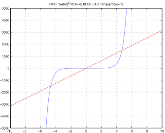
Figure 1: The procedure to find an approximation to a good initialization.

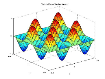
Figure 2: The initial function, trigonometric profiles.

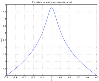
Figure 3: The section along $x$ of the solution $\psi(x,y)$.

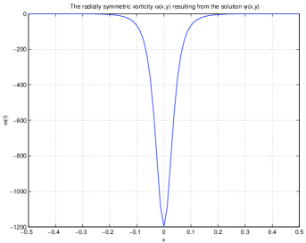
Figure 4: The vorticity, calculated from $\psi(x,y)$ obtained by integration.

In order to quantify the accuracy of integration we collect in all the domain $\left(x,y\right)$ the pairs $\left(\psi,\omega\right)$ and represent them together with the line of the nonlinear term in our equation, Fig.(5). In Fig.(6) we show the ratio of the two quantities the nonlinear term and $\omega$, as resulted from the calculated $\psi$. This ratio should be $1$. There are points close to the value $0$ where this ratio is not $1$ but, if we normalize adding an arbitrary constant to remove the possible singular cases, we notice a very good clustering of the points around the line $1$. In addition, we represent the scatterplot of the pairs ($\omega$, magnitudes of nonlinear term for the $\psi$’s) and notice the close clustering around the diagonal. Other tests are possible and they indicates that the integration is very good on most of the region and good within the imposed accuracy in the regions where the quantities reach values close to $0$.

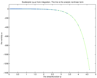
Figure 5: The scatter plot $(\psi,\omega)$, for $p=1$.

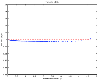
Figure 6: The ratio of $\omega$ and the nonlinear term.

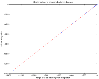
Figure 7: Scatterplot $(\omega,$ the nonlinear term), compared with the diagonal.

The contour plot of the solution is shown in Fig.(8) on the same graph with the velocity field (we have used a reduced set of data due to limitations on the EPS file). We must note that this two-dimensional integration gives a radial component of the velocity which at maximum is about $20$ times lower than the tangential one.

The tangential component of the velocity is shown in two figures (9) and (11) with the purpose of making easier the observation of the central region. The narrow dip in the center is clearly visible and its radial extension can be compared with the extension of the whole domain.

We have represented in Fig.(12) a section along the $x$ axis of the amplitude of the azimuthal component of the velocity.

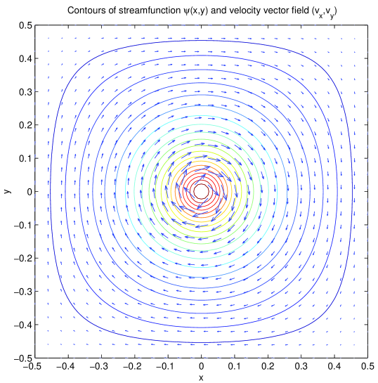
Figure 8: The contours of the scalar streamfunction $\psi(x,y)$ and the vector field $(v_{x}.v_{y})$.

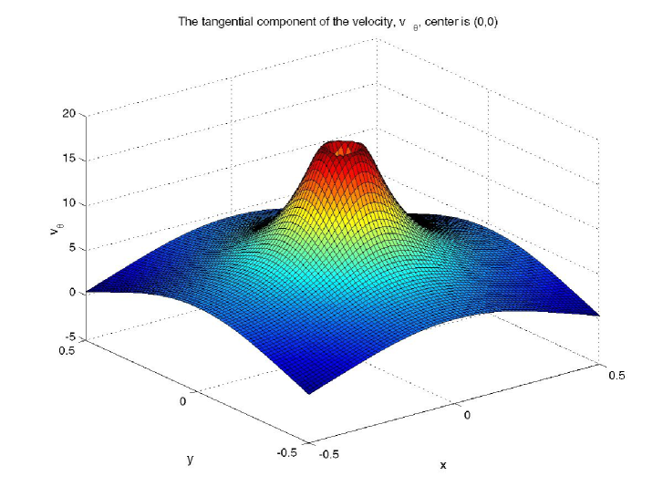
Figure 9: The tangential component $v_{\theta}(x,y)$ of the velocity vector field $(v_{x}.v_{y})$, with center at $(0,0)$.

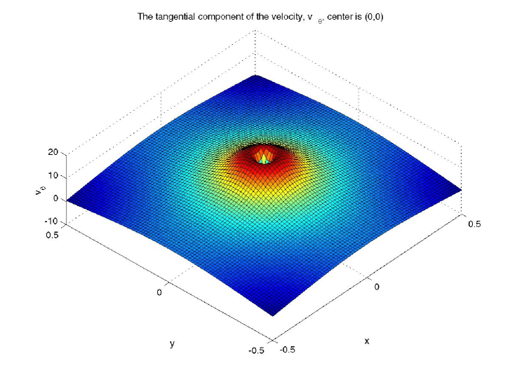
Figure 10: The tangential component $v_{\theta}(x,y)$ of the velocity vector field $(v_{x}.v_{y})$, with center at $(0,0)$ (same as 9).

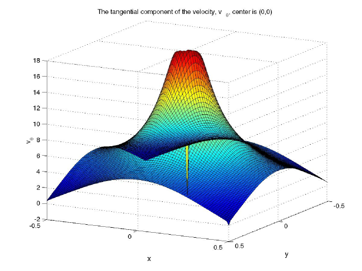
Figure 11: The tangential component $v_{\theta}(x,y)$ of the velocity vector field $(v_{x}.v_{y})$, with center at $(0,0)$ (same as 9).

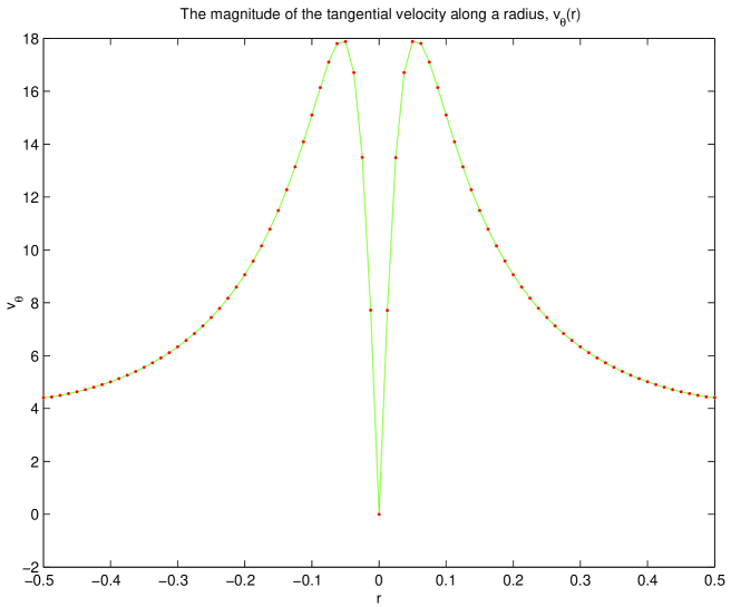
Figure 12: The magnitude of the tangential component $v_{\theta}(x,y)$, seen along a radial line. The central fast decay is clearly visible.

3.1.1 Episodic structure of two vortices

It is worth to mention that in a numerical experiment we have identified a state where two vortices have been formed, placed in symmetrical positions along the diagonal of the square domain $\left[-0.5,0.5\right]\times\left[-0.5,0.5\right]\;$with a mesh of $\left[31,31\right]$. The value of the parameter is $p=1$. The initial function is trigonometric with $k=2$ in Eq.(6) with a coefficient $\psi_{lin}=3.8$. It takes longer to obtain the solution with $0.84\times 10^{-4}$ accuracy, $389$ calls to the function. The result is in Fig.(13).

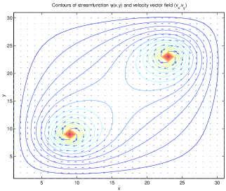
Figure 13: The contours of the scalar streamfunction $\psi(x,y)$ and the vector field $(v_{x}.v_{y}$ for a two-vortices approximative solution.

This state has been reexamined with much higher accuracy. It has taken long time to see that the final solution was again the centered vortex shown before. Therefore from the point of view of the numerical experience this state of two vortices is irrelevant. However, the persistence of this state inside the iterative search may indicate that it is close to a solution, possible less stable. We have not investigated this further. Instead we will show below a solution with four vortices.

3.1.2 Four vortices

The calculations are done for $p=1$ on meshes with various levels of details: $31$, $61$, $101$. The initial function is trigonometric with $k=3$.

The results show clearly the formation of four vortices, as shown by Fig.(15). Each of them has a structure that is similar to the one presented in Fig.(3). It is interesting to note that again the vorticity is almost zero everywhere on the domain, except a strict region around the four vortices, where it reaches very high values.

To the accuracy we have used unitl now we cannot say if the local tangential velocity presents the same very fast decay to the center of the vortex.

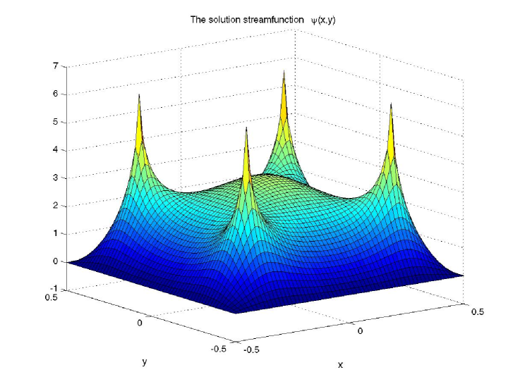
Figure 14: The scalar streamfunction $\psi(x,y)$ for a four-vortices solution.

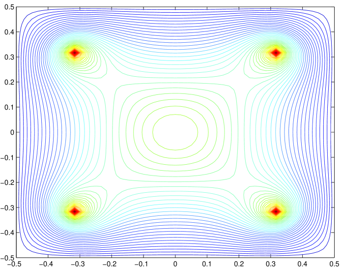
Figure 15: The contours of the scalar streamfunction $\psi(x,y)$ and the vector field $(v_{x}.v_{y})$ for a four-vortices solution.

3.1.3 Four vortices obtained at $p>1$

For $p=3$ it is also possible to obtain the four-vortex solution. The initial function is here a trigonometric combination for, $k=2$ and squared such that only positive (four) maxima are initially present, with an amplitude of about $\psi=4$.

3.1.4 The central strong decay of the tangential velocity, at $p>1$

The numerical integration is done for $p=3$ , using an initialization by a centered peak from an trigonometric function.

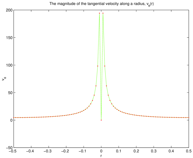
Figure 16: The magnitude of the tangential component $v_{\theta}(x,y)$, seen along a radial line. The central dip is visible but significantly narrower than at $p=1$.

We note from Fig.(16) that for larger values of the parameter $p$ there is a even more narrow zone where there is the strong decay of the tangential velocity.

3.2 Relevance of the solutions for the physics of the atmosphere

In general the space variables of the CHM equation are normalized to the intrinsic typical length of the model. In this case (atmospheric physics) are scaled with $\rho_{g}$, the Rossby radius. We note in passing, (especially for plasma physicists) that there is a major difference compared with the plasma case. In plasma, perturbations with lengths less or comparable with an ion Larmor gyroradius $k^{-1}\gtrsim\rho_{i}$ cannot be described by fluid models.

In the physics of atmosphere, the wavelengths can be much smaller

$$k\rho_{g}\gg 1$$

At very large $k\rho_{g}$ the description becomes governed by the Euler equation (see [15]).

For the numerical studies we choose

$$\left(x,y\right) \in \left[x_{\min},x_{\max}\right]\times\left[y_{\min},y_{\max}\right]$$

$$= \left[-0.5,0.5\right]\times\left[-0.5,0.5\right]$$

This means that the full domain (the side of the rectangle) is a single unit length $\rho_{g}$.

In the following we make few consideration about what we can expect as results, in the case of the atmosphere problem.

As we will notice from numerical solution, the equation produces functions with very clear similarity with the typhoon morphology. The characteristic aspect is (within the precision of these first integrations) a sharp extremum of the vorticity on $\left(0,0\right)$ which means a localised maximum of the tangential velocity $v_{\theta}$ in close proximity of the center. Since

$$v_{\theta}=\frac{d\psi}{dr}$$

the maximum at

$$r=a$$

means

$$\frac{dv_{\theta}}{dr}=\frac{d^{2}\psi}{dr^{2}}=0$$

The equation is

$$\frac{d^{2}\psi}{dr^{2}}+\frac{1}{r}\frac{d\psi}{dr}=\left(-\frac{1}{2p^{2}}\right)\sinh\psi\left(\cosh\psi-p\right)$$

We multiply by $r\,\$and we make a derivation to $r$

$$\frac{d^{2}\psi}{dr^{2}}+r\frac{d^{2}}{dr^{2}}\frac{d\psi}{dr}+\frac{d^{2}\psi}{dr^{2}}$$

$$= \left(-\frac{1}{2p^{2}}\right)\left\{\sinh\psi\left(\cosh\psi-p\right)+\right.$$

$$\left.+r\left(\frac{d\psi}{dr}\right)\left[\cosh^{2}\psi-p\cosh\psi+\sinh^{2}\psi\right]\right\}$$

We calculate this expression and the equation in the point $r=a$ defined as the point of the maximum of the tangential velocity. This means

$$r = a$$

$$\left(\frac{d^{2}\psi}{dr^{2}}\right)_{a} = 0$$

$$\left.\frac{d^{2}}{dr^{2}}\left(\frac{d\psi}{dr}\right)\right|_{a} \equiv \left.\frac{d^{2}v_{\theta}}{dr^{2}}\right|_{a}=-\alpha\;\text{where\ }\alpha>0$$

$$\psi\left(r=a\right) \equiv \psi_{0}$$

where we have introduced a notation for the value, $-\alpha<0$ of the second derivative of the tangential velocity at its maximum. For a very qualitative estimation, used in predicting shapes of solutions, we will take this as a parameter. At the point $r=a$ the equation becomes

$$\frac{1}{a}\left(\frac{d\psi}{dr}\right)_{a}=\left(-\frac{1}{2p^{2}}\right)\sinh\psi_{0}\left(\cosh\psi_{0}-p\right)$$

In the equation derivated at $r$ we replace $d\psi/dr$ with its value from the above equation and also introduce the parameter $\alpha$. Then we have

$$a\left(-\alpha\right)$$

$$= \left(-\frac{1}{2p^{2}}\right)\left\{\sinh\psi_{0}\left(\cosh\psi_{0}-p\right)\right.$$

$$+a^{2}\left(-\frac{1}{2p^{2}}\right)\sinh\psi_{0}\left(\cosh\psi_{0}-p\right)$$

$$\left.\times\left(2\cosh^{2}\psi_{0}-p\cosh\psi_{0}-1\right)\right\}$$

or

$$\frac{a\alpha\left(2p^{2}\right)}{\sinh\psi_{0}\left(\cosh\psi_{0}-p\right)}=1-\frac{a^{2}}{2p^{2}}\left(2\cosh^{2}\psi_{0}-p\cosh\psi_{0}-1\right)$$

This equation may serve to make some estimates if additional informations (or simply hints from experiments) are available. This is illustrated below.

Consider the case $p=1$

$$\frac{2a\alpha}{\sinh\psi_{0}\left(\cosh\psi_{0}-1\right)}=1-\frac{a^{2}}{2}\left(\cosh\psi_{0}-1\right)\left(2\cosh\psi_{0}+1\right)$$ (8)

A short and dirty approximation should start by using the suggestion from results of lucky simulations, where $\psi_{0}$ is few units, and $a$ is of the order $0.1$ on a domain of length $1$ in both $x$ and $y$. The second derivative of the tangential velocity must be high, shown by the plots of $v_{\theta}$. This means that it may exist a difference of magnitude of the terms, with the second term in the right hand side appearing less important. Therefore we try

$$2a\alpha\sim\sinh\psi_{0}\left(\cosh\psi_{0}-1\right)$$

In addition, we can suppose that the exponentials of negative argument are less important than those of positive argument, and simplify to

$$\exp\left(2\psi_{0}\right)\sim 8a\alpha$$

or

$$\psi_{0}\sim\frac{1}{2}\ln\left(\alpha a\right)+1$$

For an order of magnitude we may take

$$\alpha\sim\frac{\psi_{0}}{a^{3}}$$

and then

$$\psi_{0} \sim \frac{1}{2}\ln\left(\frac{\psi_{0}}{a^{2}}\right)+1$$

$$\sim \frac{1}{2}\ln\psi_{0}-\ln a+1$$

We obtain

$$\psi_{0}-1-\frac{1}{2}\ln\psi_{0}\sim-\ln a$$

$$\frac{1}{a} \sim \exp\left(\psi_{0}-1-\frac{1}{2}\ln\psi_{0}\right)$$

$$\sim \frac{1}{\sqrt{\psi_{0}}}\exp\left(\psi_{0}-1\right)$$

or

$$a\sim\frac{1}{e}\sqrt{\psi_{0}}\exp\left(-\psi_{0}\right)$$

We can see that the results are consistent, since if we take from numerical solution

$$\psi_{0}\sim 3$$

we obtain from the estimation

$$a\sim 0.032$$

which is not far from

$$a^{num}\sim 0.04$$

We must remember that the domain of integration is of length $1$ and the fact that “the radius of maximum wind” is so small, $a\sim 0.04$ , means that high accuracy is needed to describe correctly what happens close to the center. This is due to the other constraint, that the solution streamfunction $\psi\left(r\right)$ needs sufficient space to go to the constant value at “infinity” (large $r$). Any restriction of the domain of integration which would be aimed to the better description of the central region would require boundary conditions that are unknown.

There is another benefit from these very rough estimations. We can use them to determine the spatial domain that would be adequate for the search of the solution, for particular physical situations.

In order to use this rough estimation we must introduce physical units. In the following all quantities with physical dimensions have an superscript $phy$.

In atmosphere the distances are measured in $\rho_{g}$

$$a=\frac{a^{phy}}{\rho_{g}}$$

and the streamfunction is normalised with

$$\psi=\frac{\psi^{phy}}{\rho_{g}^{2}\left\langle f\right\rangle}$$

where $\left\langle f\right\rangle$ is the Coriolis parameter. This means

$$\frac{a^{phy}}{\rho_{g}}\sim\frac{1}{e}\sqrt{\frac{\psi_{0}^{phy}}{\rho_{g}^{2}\left\langle f\right\rangle}}\exp\left[-\frac{\psi_{0}^{phy}}{\rho_{g}^{2}\left\langle f\right\rangle}\right]$$

The physical parameters are (taken from [15])

The depth of the atmosphere

$$H_{0}=8\times 10^{3}\;\left(m\right)$$

The Coriolis parameter

$$\left\langle f\right\rangle=1.6\times 10^{-4}\;\left(s^{-1}\right)$$

From these parameters it results

The Rossby radius (the unit of space)

$$\rho_{g} = \frac{\left(gH\right)^{1/2}}{\left\langle f\right\rangle}$$

$$= 2\times 10^{6}\,\left(m\right)$$

The unit for the streamfunction is

$$\rho_{g}^{2}\left\langle f\right\rangle=6.4\times 10^{8}\;\left(m^{2}/s\right)$$

The unit for vorticity

$$\left\langle f\right\rangle=1.6\times 10^{-4}\;\left(s^{-1}\right)$$

For example, using these parameters, it results that we have integrated on a spatial domain of length $L$ (in other words: we have imposed that the streamfunction becomes equal to $\psi_{b}^{\left(1,2\right)}$ on the boundaries of a square with side length $L$)

$$L \equiv x_{\max}-x_{\min}=1$$

$$L^{phy} = 1\times\rho_{g}\sim 2\times 10^{6}\;\left(m\right)=2000\;\left(km\right)$$

and the diameter $d$ of the eye of the typhoon results

$$d = 2\times a=0.08$$

$$d^{phy} \sim 0.08\rho_{g}=128\;\left(km\right)$$

In the Ref.[24] it is reproduced a plot of an observation made on the profile of the vorticity, in Fig.1a. The plot indicates a maximum value of about $250\times 10^{-4}\left(s^{-1}\right)$. The vorticity we obtain is larger (of the order of $1000\times 10^{-4}$). This shows that the absence of the third dimension in our model and of the viscous effects have a serious influence on the physical quantities. They should be somehow accounted for by renormalizing the two-dimensional model at the initial stage. For example, in the case of the plasma vortex, a change of the space scale results from the presence of a translational motion combined with the density gradient. This remains to be studied.

4 Summary

We again underline that this equation is very difficult to solve, although it requires reasonable computer resources. The main problem is the complexity of the space of solutions and the need to explore carefully much of this space in order to establish the basins of attraction. We are not able at this moment to connect in some practically useful way the sharp transitions between the attractors with the stability of the solutions.

It seems that the solution where the streamfunction $\psi\left(x,y\right)$ is approximately radially symmetric, strongly peaked in origin, is a significant attractor, at the level of this very sensitive equation. It presents the particularity that the vorticity is practically zero for almost all spatial domain and is strongly localised, almost singular, close to the maximum. The aspect of this solution is very similar to the two-dimensional image of a typhoon.

We have several arguments in favor of the conclusion that our equation (1) may represent the hydrodynamic part of the atmospheric vortex. We mention some of them.

1. The profile of the magntitude of the tangential velocity, as represented in Fig.2 of Ref. [22] is very similar to our Fig.12. This is also confirmed by similarity with the Fig.1a from Ref( [23]);

2. The profile of the vorticity $\omega$ shown in our Fig.4 is very similar to Fig.1a from Ref.[24];

3. We note that in  a series of reported numerical simulations, the tendency of the fields is to evolve toward profiles that are very close to those shown in our figures 3, 4 and 12. For example, the Fig.7a and b of Ref.[24] show the evolution of the azimuthal mean of the vorticity and tangential velocity from initial profiles which correspond to a narrow ring of vorticity to profiles that show clear ressemblance with our figures 4 and 12 or 9. The same striking evolution to profiles similar to ours appears in Figs.7 a and b of the same Reference. We have investigated whether a radially annular profile of vorticity can be a solution of our equation (1). The result is negative, which may explain why such an initial profile evolves to either a set of vortices (vortex-crystal) or to a centrally peaked structure as in Fig.9.

4. The four vortices represented in Figure 4a of the Ref. [24] as the late stage of the evolution obtained from numerical simulation of vorticity, is clearly similar to our figure 15.

5. We obtain a good consistency between our quantitative results for an atmospheric vortex (using most elementary input information) and the values measured or obtained in numerical simulations, at least for some of the quantities.

A large database on typhoons can be found in [28]. The similarity is striking and it suggests that further work with this equation is worth to be done.

The numerical simulations we have taken as a comparison are very complex. In general, the physics of the typhoons is very complex and includes hydrodynamics and thermic aspects, with many additional elements: precipitation, viscosity, etc. In no way we do not claim that this equation can represent this complexity. It appears however useful as a description of the regimes where the hydrodynamical processes are dominating and have reached stationarity.

Acknowledgments. We are very grateful to Professor David Montgomery for many discussions on a wide spectrum of problems. We thank Dr. L. Weimann for his kind help on the GIANT code.

This work has been partly supported by a grant from the Japan Society for the Promotion of Science. The authors are very grateful for this support and for the hospitality of Professor S.-I. Itoh and of Professor M. Yagi.

5 Appendix A : The structure of a radial solution near $r=0$ and $r=\infty$

The equation we discuss is

$$\Delta\psi+\frac{1}{2p^{2}}\sinh\psi\left(\cosh\psi-p\right)=0$$

Other members of the family of equations (parametrized by solutions of the $2D$ Laplace equation) will be examined separately. Their importance stems from the fact that they can provide, in principle, azimuthal trigonometric variation, as for example the Larichev-Reznik modon.

5.1 The behavior near $r=0$

Close to the origin, in a purely radial form, it is

$$\frac{d^{2}\psi}{dr^{2}}+\frac{1}{r}\frac{d\psi}{dr}+\left(\frac{1}{2p^{2}}\right)\sinh\psi\left(\cosh\psi-p\right)=0$$

where $r$ is measured in $\rho_{s}$.

We take an expansion with only even powers of $r$ close to the origin

$$\psi\sim a_{0}+a_{2}r^{2}+a_{4}r^{4}+a_{6}r^{6}+...$$

Then, for small $r$;

$$\frac{d\psi}{dr} = 2a_{2}r+4a_{4}r^{3}+6a_{6}r^{5}...$$

$$\frac{1}{r}\frac{d\psi}{dr} = 2a_{2}+4a_{4}r^{2}+6a_{6}r^{4}...$$

$$\frac{d^{2}\psi}{dr^{2}}=2a_{2}+12a_{4}r^{2}+30a_{6}r^{4}+...$$

$$\sinh\left(a_{0}+a_{2}r^{2}+a_{4}r^{4}+...\right)$$

$$= \sinh a_{0}$$

$$+\left(a_{2}r^{2}+a_{4}r^{4}+...\right)\cosh a_{0}$$

$$+\frac{1}{2}\left(a_{2}^{2}r^{4}+...\right)\sinh a_{0}+...$$

$$\cosh\left(a_{0}+a_{2}r^{2}+a_{4}r^{4}+...\right)$$

$$= \cosh a_{0}$$

$$+\left(a_{2}r^{2}+a_{4}r^{4}+...\right)\sinh a_{0}$$

$$+\frac{1}{2}\left(a_{2}^{2}r^{4}+...\right)\cosh a_{0}+...$$

Introducing the notations

$$U \equiv a_{2}r^{2}+a_{4}r^{4}+...$$

$$V \equiv \frac{1}{2}\left(a_{2}^{2}r^{4}+...\right)$$

$$\sinh\psi\left(\cosh\psi-p\right)$$

$$= \left(\sinh a_{0}+U\cosh a_{0}+V\sinh a_{0}\right)$$

$$\times\left(\cosh a_{0}-p+U\sinh a_{0}+V\cosh a_{0}\right)$$

$$= \sinh a_{0}\left(\cosh a_{0}-p\right)$$

$$+U\left(\sinh^{2}a_{0}+\cosh^{2}a_{0}-p\cosh a_{0}\right)$$

$$+V\left(2\cosh a_{0}\sinh a_{0}-p\sinh a_{0}\right)$$

$$+U^{2}\left(\sinh a_{0}\cosh a_{0}\right)$$

$$+V^{2}\left(\sinh a_{0}\cosh a_{0}\right)$$

$$+UV\left(\cosh^{2}a_{0}+\sinh^{2}a_{0}\right)$$

$$+...$$

We collect the various degrees of $r^{\alpha}$

$$q_{0}+q_{2}r^{2}+q_{4}r^{4}+...$$

$$q_{0}=\sinh a_{0}\left(\cosh a_{0}-p\right)$$

$$q_{2}=a_{2}\left(\sinh^{2}a_{0}+\cosh^{2}a_{0}-p\cosh a_{0}\right)$$

$$q_{4} = a_{4}\left(\sinh^{2}a_{0}+\cosh^{2}a_{0}-p\cosh a_{0}\right)$$

$$+\frac{1}{2}a_{2}^{2}\left(2\cosh a_{0}\sinh a_{0}-p\sinh a_{0}\right)$$

$$+a_{2}^{2}\left(\sinh a_{0}\cosh a_{0}\right)$$

Returning to the differential operator

$$\frac{d^{2}\psi}{dr^{2}}+\frac{1}{r}\frac{d\psi}{dr}$$

$$= 2a_{2}+12a_{4}r^{2}+30a_{6}r^{4}+...$$

$$+2a_{2}+4a_{4}r^{2}+6a_{6}r^{4}...$$

$$= 4a_{2}+16a_{4}r^{2}+36a_{6}r^{4}+...$$

We now identify the expressions corresponding to the same degrees of $r$,

$$4a_{2}+16a_{4}r^{2}+36a_{6}r^{4}+...$$

$$+\left(\frac{1}{2p^{2}}\right)\left(q_{0}+q_{2}r^{2}+q_{4}r^{4}+...\right)$$

$$= 0$$

with the equalities

$$4a_{2}+\left(\frac{1}{2p^{2}}\right)q_{0}=0$$

$$16a_{4}+\left(\frac{1}{2p^{2}}\right)q_{2}=0$$

$$36a_{6}+\left(\frac{1}{2p^{2}}\right)q_{4}=0$$

The equations from which we derive the coefficients of the expansion become

$$4a_{2}+\left(\frac{1}{2p^{2}}\right)\sinh a_{0}\left(\cosh a_{0}-p\right)=0$$

$$16a_{4}+\left(\frac{1}{2p^{2}}\right)a_{2}\left(\sinh^{2}a_{0}+\cosh^{2}a_{0}-p\cosh a_{0}\right)=0$$

$$36a_{6}+\left(\frac{1}{2p^{2}}\right)\left[a_{4}\left(\sinh^{2}a_{0}+\cosh^{2}a_{0}-p\cosh a_{0}\right)\right.$$

$$+\frac{1}{2}a_{2}^{2}\left(2\cosh a_{0}\sinh a_{0}-p\sinh a_{0}\right)$$

$$\left.+a_{2}^{2}\left(\sinh a_{0}\cosh a_{0}\right)\right]$$

$$= 0$$

We see that if we take

$$a_{0}=0$$

then this will vanish all the other coefficients

$$a_{2} = 0$$

$$a_{4} = 0$$

$$a_{6} = 0,...$$

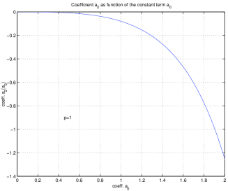
Figure 17: Coefficient $a_{2}$ for $p=1$.

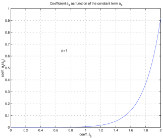
Figure 18: Coefficient $a_{4}$ for $p=1$.

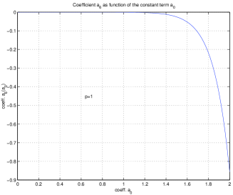
Figure 19: Coefficient $a_{6}$ for $p=1$.

Consider the value of the constant

$$p=1$$

and we choose the main coefficient of the expansion close to $r=0$ to be

$$a_{0}=1$$

Then

$$a_{2} = -0.0798$$

$$a_{4} = 0.0055$$

$$a_{6} = -0.000439$$

But the coefficients, as shown in the Figures, are very rapidly growing in absolute value.

We conclude that any attempt to identify the solution starting from few terms expansion around $r=0$ will be imprecise.

5.2 The behavior at infinity

At $r\rightarrow\infty$ we expect that the function approaches zero in the case where $p=1$ or approaches one of the roots of the equation

$$\cosh\psi-p=0$$ (9)

for $p>1$. The case where $\psi\rightarrow 0$ will be treated below. We note, for the case $p>1$ that the solutions of the Eq.(9) are

$$\psi_{b}^{\left(1\right)} = \ln\left(p+\sqrt{p^{2}-1}\right)$$

$$\psi_{b}^{\left(2\right)} = \ln\left(p-\sqrt{p^{2}-1}\right)$$

5.2.1 The case $p=1$

This requires that $\psi\rightarrow 0$ at $r\rightarrow\infty$.

Change the variable

$$r\rightarrow\frac{1}{x}$$

$$\frac{d}{dr}=\frac{dx}{dr}\frac{d}{dx}=-\frac{1}{r^{2}}\frac{d}{dx}=-x^{2}\frac{d}{dx}$$

$$\frac{d^{2}}{dr^{2}} = \frac{d}{dr}\left(\frac{d}{dr}\right)=-x^{2}\frac{d}{dx}\left(-x^{2}\frac{d}{dx}\right)$$

$$= -x^{2}\left(-2x\frac{d}{dx}-x^{2}\frac{d^{2}}{dx^{2}}\right)$$

$$= 2x^{3}\frac{d}{dx}+x^{4}\frac{d^{2}}{dx^{2}}$$

The function

$$\psi\rightarrow 0$$

$$\left(\frac{1}{2p^{2}}\right)\sinh\psi\left(\cosh\psi-p\right) \rightarrow \left(\frac{1}{2p^{2}}\right)\left(\psi-\frac{\psi^{3}}{6}\right)\left(1-p-\frac{\psi^{2}}{2}\right)$$

$$= \frac{1-p}{2p^{2}}\psi$$

$$+\frac{1}{2p^{2}}\left(-\frac{1}{2}-\frac{1-p}{6}\right)\psi^{3}+...$$

For

$$p = 1$$

$$\left(\frac{1}{2p^{2}}\right)\sinh\psi\left(\cosh\psi-p\right) \rightarrow -\frac{1}{4}\psi^{3}$$

Then the equation becomes

$$\left(2x^{3}\frac{d}{dx}+x^{4}\frac{d^{2}}{dx^{2}}\right)\psi$$

$$+\left(-x^{2}\frac{d}{dx}\right)\psi$$

$$+\frac{1-p}{2p^{2}}\psi+\frac{1}{2p^{2}}\left(-\frac{1}{2}-\frac{1-p}{6}\right)\psi^{3}$$

$$= 0$$

This can be approximated at

$$x\rightarrow 0$$

$$-x^{2}\frac{d\psi}{dx}=\alpha\psi+\beta\psi^{3}$$

or

$$\frac{d\psi}{\alpha\psi+\beta\psi^{3}}=-\frac{dx}{x^{2}}=d\left(\frac{1}{x}\right)=dr$$

For

$$p=1$$

$$\alpha = 0$$

$$\beta = -\frac{1}{4}$$

then

$$\left(-4\right)\frac{d\psi}{\psi^{3}}=dr$$

$$\psi\sim\sqrt{\frac{2}{r}}$$

We note however that in this case the vorticity is

$$\omega = \Delta\psi$$

$$\sim r^{-5/2}$$

We would like to have a vanishing vorticity at infinity with a faster decay.

The above calculations seem to suggest that for purely radial structure we need to consider the differential equation which is derived for a different choice of the Laplacean equation, as it is explained in the main text.

5.2.2 The case $p>1$

One possibility, for

$$p>1$$

$$\alpha\equiv\frac{1-p}{2p^{2}}<0$$

$$\psi\sim\exp\left(-\left|\alpha\right|r\right)$$

This gives

$$\omega = \Delta\psi$$

$$\sim \left(-\left|\alpha\right|\right)\frac{\exp\left(-\left|\alpha\right|r\right)}{r}+\alpha^{2}\exp\left(-\left|\alpha\right|r\right)$$

with a fast decay. This situation is worth to be examined numerically.

6 Appendix B : various forms of the initial conditions

6.1 The ring-type

The initial form of the function has the form

$$\psi_{0}=A\exp\left(-sr^{2}\right)\left[1-\kappa\exp\left(-qr^{4}\right)\right]$$

We look for the maximum

$$\frac{d\psi_{0}}{dr} = \left(-2sr\right)\exp\left(-sr^{2}\right)\left[1-\kappa\exp\left(-qr^{4}\right)\right]$$

$$+\exp\left(-sr^{2}\right)\left(4qr^{3}\right)\kappa\exp\left(-qr^{4}\right)$$

$$= 0$$

and we take the maximum to be placed at

$$r=a$$

which is considered to approximate the center line of the ring. The equation becomes

$$\left(2s\kappa+4\kappa qa^{2}\right)\exp\left(-qa^{4}\right)=2s$$

$$\kappa\exp\left(-qa^{4}\right)=\frac{1}{1+2a^{2}\left(q/s\right)}$$

The other condition is that the maximum of the function $\psi_{0}$ at $r=a$ equals a prescribed value,

$$\psi_{0}\left(r=a\right) = \psi_{c}$$

$$A\exp\left(-sa^{2}\right)\left[1-\kappa\exp\left(-qa^{4}\right)\right] = \psi_{c}$$

The initial condition is introduced in the following way. We take $q$, $a$, $\kappa$ and $\psi_{c}$ as input parameters and determine the other two, $s$ and $A$ from the equations

$$s=\frac{2a^{2}q}{\kappa\exp\left(-qa^{4}\right)-1}$$

$$A=\frac{\psi_{c}}{\exp\left(-sa^{2}\right)\left[1-\kappa\exp\left(-qa^{4}\right)\right]}$$

Now the initial function will be

$$\psi_{initial}\left(r\right) = \psi_{0}+\psi_{b}^{\left(1,2\right)}$$

$$= \psi_{b}^{\left(1,2\right)}+$$

$$+A\exp\left(-sr^{2}\right)\left[1-\kappa\exp\left(-qr^{4}\right)\right]$$

i.e. the function just determined is placed on the constant background of the value at the boundary, calculated form the condition that the vorticity is zero at infinity.

This class of initial functions is characterised by an annular shape, with exponential decay for $r\rightarrow\infty$, with a minimum in the region around $r=0$ of depth that can be fixed by varying $\kappa$. For $\kappa=1$ the function is zero on the symmetry axis and rises slowly (due to $r^{4}$) toward the maximum at $r=a$.

In order to narrow the space of parameters we require the approximative equality between the vorticity amplitude at the ring with the nonlinear term

$$\omega \sim -\frac{2}{\delta^{2}}\psi_{c}$$

$$\sim -\frac{1}{2p^{2}}\sinh\left(\psi_{c}+\psi_{b}^{\left(1,2\right)}\right)\left[\cosh\left(\psi_{c}+\psi_{b}^{\left(1,2\right)}\right)-p\right]$$

(Here $\delta$ is the width of the ring shape). These two quantities are compared in graphical plot for a range of values of the parameter $\psi_{c}$, using a Matlab script. This is far from an exact procedure but helps to generate reasonable ranges for the input parameters.

The conclusion after many trials using this procedure and its initial function forms can be described as follows.

In most of the cases the central region is corrected and shifted to a maximum. In the cases $p=1$ the central region which is started with a deppressed level is rised and a strong peaked form is generated, as in the cases where the initialization consists of a maximum on center (for example a Gaussian form). For $p>1$ the run evolves in some cases to the formation of separate maxima placed symmetrically on a ring, having sharp maxima. The central region is decreased in amplitude to a somehow flat region. The region outside the ring is evolving to a state which corresponds with very good precision, to

$$\omega\sim 0$$

on the rest of the domain to the periphery.

6.2 Flat central region for $\psi\left(r\right)$

We take the central region

$$0<r<r_{flat}$$

with a fixed, constant value

$$\psi\left(r\right)=\psi_{c}$$

where $\psi_{c}$ is one of the roots of the equation $\cosh\psi-p=0$. At the edge we take another fixed value,

$$\psi=\psi_{b}$$

with $\psi_{b}$ the other, smaller root of the equation.

In between, we take

$$\psi\left(r\right)=\psi_{1}-A\ln\left(r\right)$$

$$A=\frac{\psi_{c}-\psi_{b}}{\ln\left(r_{flat}/r_{c}\right)}$$

$$\psi_{1}=\psi_{c}+A\ln\left(r_{flat}\right)$$

The value $r_{c}$ is

$$r_{flat}<r_{c}<0.5$$

represents the value where where we stop the decay of the function with logarithm profile and put $\psi=\psi_{b}$. This is

$$r_{flat} = 0.1$$

$$r_{c} = 0.35\cdots 0.45$$

The parameter $p=1.3$.

The result of these calculations is as follows. For small mesh, the evolution is clearly toward the suppression of the smoothly decaying part, letting a sort of cylinder in the center, with radius $r_{flat}$, with the high value equal to $\psi_{c}$ and the rest seems to go progressively to $\psi=\psi_{b}$. The vorticity is singular, around $r=r_{flat}$. The vorticity is positive and negative, with high values, singular in a narrow ring.

For this cylindrical-rod profile of the streamfunction $\psi\left(r\right)$, the velocity is very localised, as a very narrow ring, all its values are positive. The velocity grows from zero, keeps always the same direction on $\theta$ and then decays to zero value, after the width of the ring. The vorticity is also sharply limitted here, but it has positive and negative values on interior half of the ring and respectively on the exterior half of the ring.

The same shrinking to the cylindrical column happens when we take the maximum of $\psi$ (in the central flat region) as

$$\psi\left(r\right)=0$$

which is the other possibility that the equation is verified for constant value of $\psi$.

References

- [1] J. G. Charney, Geophys. Public. Kosjones Nors. Videnshap. Akad. Oslo, 17 (1948) 3.
- [2] A. Hasegawa and K. Mima, Phys. Fluids 21 (1978) 87.
- [3] D. Montgomery, W.H. Mathaeus, W.T. Stribling, D. Martinez and S. Oughton, Phys. Fluids A4 (1992) 3
- [4] D. Fyfe, D. Montgomery and G. Joyce, J. Plasma Phys. 17, 369 (1976).
- [5] R. H. Kraichnan and D. Montgomery, Rep. Prog. Phys. 43, 547 (1980)
- [6] D. Montgomery and G. Joyce, Phys. Fluids 17, 1139 (1974)
- [7] D. Montgomery, L. Turner and G. Vahala, J. Plasma Phys. 21, 239 (1979)
- [8] G. Joyce and D. Montgomery, J. Plasma Phys. 10, 107 (1973)
- [9] R.A. Smith, Phys. Rev. A43, 1126 (1991).
- [10] C. E. Seyler, J. Plasma Physics 56 (1996) 553.
- [11] S. Li, D. Montgomery and W. B. Jones, Theor. Comput. Fluid Dynamics 9 (1997) 167.
- [12] W. Horton, T. Tajima, T. Kamimura, Phys. Fluids 30 (1987) 3485.
- [13] R. Kinney, J. C. McWilliams and T. Tajima, Phys. Plasmas 2 (1995) 3623.
- [14] R. Kinney, T. Tajima, J. C. McWilliams and N. Petviashvili, Phys. Plasmas 1 (1994) 260.
- [15] W. Horton and A. Hasegawa, Chaos 4 (1994) 227.
- [16] P. H. Diamond, E.-J. Kim, Physics of Plasmas, 2002.
- [17] F. Spineanu and M. Vlad, Phys. Rev.E 67 (2003) 046309.
- [18] F. Spineanu and M. Vlad, arxiv.org/physics/0501020 (submitted for publication).
- [19] F. Spineanu, M. Vlad, K. Itoh and S.-I. Itoh, Japan Journ. of Plasma Research, 2005.
- [20] F. de Rooij, P. F. Linden and S. B. Dalziel, J. Fluid Mech. 383 (1999) 249.
- [21] H. E. Willoughby and P.G. Park, Bull. American Meteorological Society, 77 (1996) 543.
- [22] Y. Wang and C.-C. Wu, Meteorol. Atmos. Phys. 87 (2004) 257.
- [23] P.D. Reasor and M. T. Montgomery, J. Atmos. Sci. 58 (2001) 2306.
- [24] J. P. Kossin and W. H. Schubert, J. Atmos. Sci. 58 (2001) 2196.
- [25] B. E. McDonald, J. Computational Phys. 16 (1974) 360.
- [26] D. Montgomery, private communication.
- [27] U. Nowak and L. Weimann, GIANT A software package for the numerical solution of very large systems of highly nonlinear equations, Konrad-Zuse-Zentrum fur Informationtechnik Berlin, Technical Report TR 90-11 (1990).
- [28] Typhoon database at the web address: http://agora.ex.nii.ac.jp/digital-typhoon.