Enhancing robustness and immunization in geographical networks

Abstract

We find that different geographical structures of networks lead to varied percolation thresholds, although these networks may have similar abstract topological structures. Thus, the strategies for enhancing robustness and immunization of a geographical network are proposed. Using the generating function formalism, we obtain the explicit form of the percolation threshold $q_{c}$ for networks containing arbitrary order cycles. For 3-cycles, the dependence of $q_{c}$ on the clustering coefficients is ascertained. The analysis substantiates the validity of the strategies with an analytical evidence.

Complex networks (see reviews CN-review ) provide powerful tools to investigate complex systems in nature and society. The properties of complex systems are affected by the geographical distribution of the components. For example, routers of the Internet internet and transport networks transport lay on the two-dimensional surface of the globe; world-wide airport network is confined by the geography airport ; neuronal networks in brains neuron occupy three-dimensional space. Thus it is helpful to study the geographical complex networks BBPV:2004 ; lesf ; snsf ; GCN-other ; GCN-yang ; sandpile .

From the abstract geometrical point of view, an abstract set can describe a general system. When it is equipped with some geometrical structures, the set can further describe a specified system. So, an abstract topological network is an abstract set that consists of nodes and links. A metric can be added to the abstract topological network, the metric could be arbitrary, not necessarily the Euclidean metric BBPV:2004 . Embedding a particular abstract topological network, into a suitable metric space provides a method to add a metric.

In this paper, the problem of percolation thresholds in geographical networks is studied. Three types of geographical networks are investigated: the normal model lesf ; snsf , the hollow model and the concentrated model. By extensive numerical simulations, we found that the percolation threshold $q_{c}$ (the point that a spanning connected cluster emerges) for these models satisfies: $q_{c}$(concentrated)$>$$q_{c}$(normal)$>$$q_{c}$(hollow). Based on these results, we suggest a strategy (hollowing) for enhancing robustness and a strategy (concentrating) for immunization of geographical networks. The different geographical networks have different distribution of cycles. The geographical dependence of the percolation threshold is investigated by the generating function process in abstract networks containing cycles.

Based on the lattice embedded model lesf , the networks are generated as follows: each node in an $L\times L$ lattice with periodic boundary conditions is assigned a degree quota $k$, drawn from the prescribed degree distribution. Here, scale-free ($P(k)\sim k^{-\lambda},m\leqslant k$) and exponential ($P(k)\sim e^{-k/k_{0}},m\leqslant k$) degree distributions are considered, where $m$ is the minimum degree a node can have. (a) The normal case [lattice embedded scale-free (LESF) or lattice embedded exponential (LEE)]: A node $i$ connects to its closest neighbors until its degree $k_{i}$ is realized, or up to a cutoff distance $A\sqrt{k_{i}}$, where $A$ is large enough to ensure that almost all the degree quotas can be fulfilled. (b) The hollow case [hollow LESF (HLESF) or hollow LEE (HLEE)]: similar to the normal case, except that a node $i$ has probability $p$ to be forbidden to connect its first $n$ nearest neighbors. (c) The concentrated case: $A$ is set smaller than that in the normal case. The process is repeated throughout all the nodes in the lattice. For the hollow case, when the network degenerates to a lattice and $n$ is small, it becomes similar to the tunneling effect on Euclidean lattices GS1995 . In the following simulations, we choose $A=7$, $n=8$, and $p=1$; network size $N=10^{6}$, minimum degree $m$ is $4$ for scale-free networks and $1$ for exponential networks, and all the data are averaged over $1000$ ensembles, unless otherwise specified.

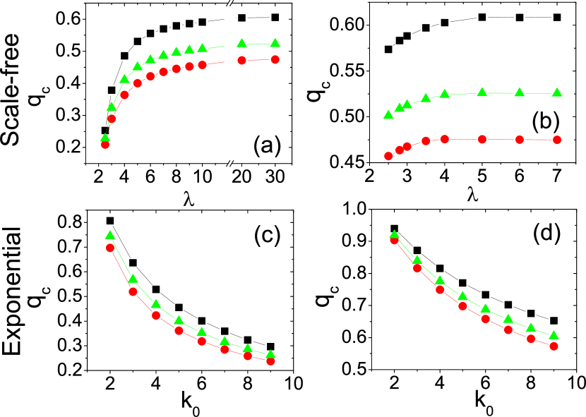
Figure 1: (Color online) Percolation thresholds of the networks for both random failures (left panels) and intentional attacks (right panels). In each subgraph squares represent for normal lattice embedded networks, triangles for hollow lattice embedded networks with $p=0.5$ and circles for $p=1$.

The algorithms of Newman and Ziff algorithm is performed to calculate the threshold $q_{c}$, which is defined as the point where the differential of the size of the largest cluster as a function of occupying probability $q$ maximizes. The definition is equivalent to the usual definition by the emergence of a spanning cluster for large network size limit threshold . Figure 1 shows a clear drop of the percolation threshold $q_{c}$ in the hollow networks than in the normal networks. So the robustness can be enhanced by the model. The size effect (scale-free degree distribution) is demonstrated in Fig. 2. The LESF and even the HLESF networks also have non-zero percolation thresholds for $\lambda\in(2,3)$, the results are consisitent with Ref. threshold . Again, the drop in $q_{c}$ for hollow networks is apparent.

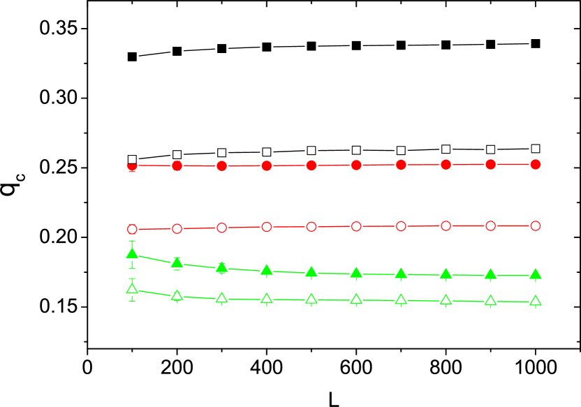
Figure 2: (Color online) Random percolation threshold $q_{c}$ vs network side length $L$ for the LESF model (filled symbols) and the HLESF model (empty symbols) for different $\lambda$: Squares for $\lambda=2.8$ , circles for $\lambda=2.5$, and triangles for $\lambda=2.3$. Each data is the result of averaging $10^{4}$ network realizations.

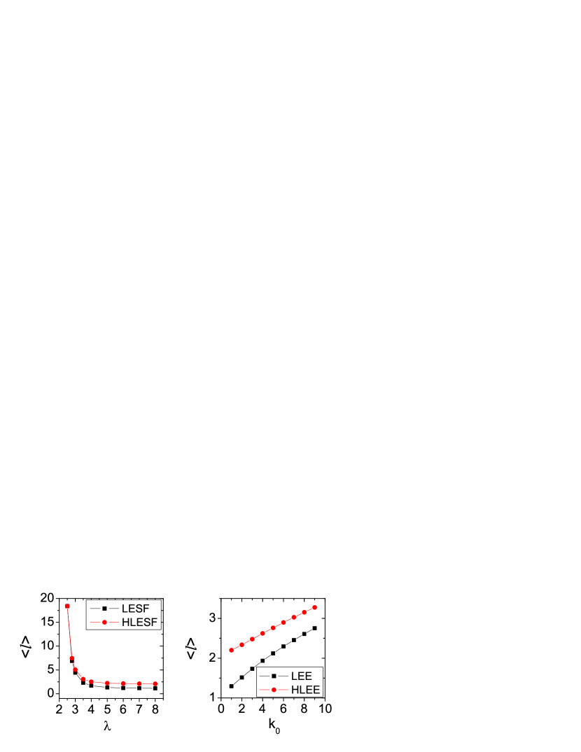
Figure 3: (Color online) The average spatial length of connections of the normal networks (squares) and hollow networks (circles) for scale-free degree distribution (a) and exponential degree distribution (b).

The amendment in hollow networks is small in the physical space. As Fig. 3 shows, the average spatial length $\left\langle l\right\rangle$ of the edges for the hollow networks dose not increase much compared with the normal networks, for small $\lambda$ or large $k_{0}$. As the average degree $\left\langle k\right\rangle$ becomes larger, the difference between $\left\langle l\right\rangle$ decreases. In the limit case, the difference goes to $0$. While the cost of constructing hollow networks still remains low, they are more robust than the normal models. Under the same conditions, the hollow networks have significant lower percolation thresholds.

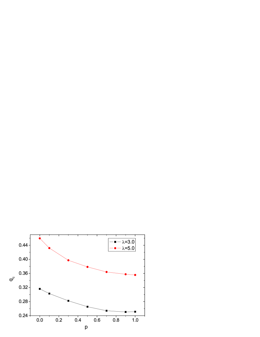
Figure 4: (Color online) Random percolation thresholds vs the rearrange probability for LESF networks, $n=8$.

Based on the above observations, we propose a hollowing strategy to enhance the robustness of geographical networks. For each node in a geographical networks, we introduce a probability $p$ to cut down the edges that linked to its first $n$ nearest neighbors, then to reconnect further nodes in the geographical distance. In this case, the degree distribution $P(k)$ deviates a little for small $k$, i.e., around about $10$. This only causes a variation in percolation thresholds of a much smaller magnitude. Figure 4 demonstrates the efficiency of the hollowing strategy for LESF networks. The percolation threshold drops about $0.1$ with $n=8$, namely, it needs 10 percent less nodes of the network to maintain a spanning cluster. This can have significant effect to prevent the network from breakdown when the network undergoes a serious crisis and is losing its global function.

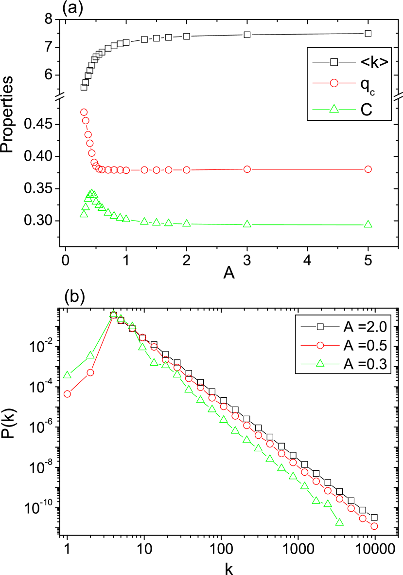
Figure 5: (Color online) Properties of concentrated networks. (a): Squares are the average degrees, circles are the random percolation thresholds, and triangles are the clustering coefficients. (b): The actual degree distribution for three typical $A$ values. The data are log-binned. The assigned degree distribution is scale-free, with $\lambda=3.0$.

For concentrated cases, we study the concentrated scale-free networks since the problem mainly concerns with immunization strategies YCLai . The long-range links (for large $A$) in the LESF model are different from those in the small-world model sw . In the LESF model, a node $i$ first tries to connect to its nearest neighbors; if they have already fulfilled their degree quotas, this node has to try further nodes until up to the cutoff distance $A\sqrt{k_{i}}$. The long-range links in the LESF model are still somewhat local. As far as $A$ is large enough to ensure that almost all the nodes’ degree quotas are fulfilled, the network properties depend little on $A$, as shown in Fig. 5(a). However, as $A$ decreases, more and more long-range links are prohibited lesf . The network becomes more localized, thus the clustering coefficient increases while the average degree decreases a little. As $A$ is approximately larger than $0.5$, most of the nodes’ degree quotas are still fulfilled except the nodes with large degree quotas. Thus the network structure remains mainly unchanged, and the percolation thresholds remains almost the same. As $A$ decreases further ($A<0.5$), a large portion of the degree quotas of nodes cannot be fulfilled. Figure 5(b) shows a serious degree cutoff ($A=0.3$), where the steps in the degree distribution come from the symmetry of the 2D lattice. Thus the network structure becomes seriously deteriorated: the average degree decreases sharply, the clustering coefficient drops; the percolation threshold increases rapidly. These effects indicate that the concentrated networks, are much easier to be immunized. This is indeed the case that, during an epidemic, most people are staying home to seclude from the infection.

To better understand the numerical results, we employ the generating function method to determine the percolation threshold for networks with different clustering properties. Here the clustering properties can be simply depicted by the clustering coefficient, which counts for the triangles (3-cycles) in the network, and it can also be represented by the number of rectangles (4-cycles), and generally by the number of $L$-cycles. In the following, a general relation of the percolation threshold $q_{c}$ and the number of $L$-cycles for a random network with arbitrary degree distribution is determined. As an example, the dependence of $q_{c}$ on the clustering coefficient is obtained.

For uniform occupations (or random failures), the percolation threshold of random tree-like networks is $q_{c}=\left\langle k\right\rangle/\left\langle k(k-1)\right\rangle$ cohenqc ; genth . It could be obtained by the condition that the average cluster size diverges, or equivalently, the average size of clusters that reached by following an edge diverges. A real network is usually clustered and contains certain amount of cycles. If the number of cycles is small, (e.g. each node belongs to at most one cycle) the generating function process can be extended to cope with the random percolation problem.

For a uniform occupation probability $q$, the generating function for the probability of the number of outgoing edges of a target node reached by following a randomly chosen edge on a clustered network remains the same as that of the random tree-like networks genth ; genth1 : $F_{1}(x)=\frac{q}{\left\langle k\right\rangle}\sum kP(k)x^{k-1}$. However, if an outgoing edge is not independent, i.e., it is terminated to a node that has already been visited (having no contribution for reaching new nodes), the node with degree $k$ will only have $k-2$ independent outgoing edges. Thus it is convenient to define

$$F_{1}^{(1)}(x)=\frac{q}{\left\langle k\right\rangle}\sum kP(k)x^{k-2}=x^{-1}F_{1}(x),$$

as the generating function of the number of outgoing edges reaching new nodes for such a target node.

Let $H_{1}(x)$ be the generating function of the size distribution of the cluster that reached by following an edge, by following $2$ independent edges, the cluster size distribution is generated by $H_{1}(x)^{2}$. But if the $2$ edges originate from a common node and belong to an $L$-cycle, the generating function should be $H_{1}^{(l_{1})}(x)H_{1}^{(l_{2})}(x)$, where $l_{1}=[(L-1)/2]$, $l_{2}=L-1-l_{1}$. $\left[g\right]$ is Gauss’ function which returns the integer part of $g$. $H_{1}^{(l)}(x)$ is the generating function for the size distribution of the clusters that is reached by an edge and has one edge terminated after $l$ steps, and satisfies an iterative relation

$$H_{1}^{(l)}(x)=1-F_{1}(1)+xF_{1}^{(1)}(H_{1}(x))H_{1}^{(l-1)}(x),$$

where the terminal condition $H_{1}^{(1)}(x)$ is

$$H_{1}^{(1)}(x)=1-F_{1}(1)+xF_{1}^{(1)}(H_{1}(x)).$$

Thus

$$H_{1}^{(l)}(x) = \left(1-F_{1}(1)\right)\frac{1-\left(xF_{1}^{(1)}(H_{1}(x))\right)^{l}}{1-xF_{1}^{(1)}(H_{1}(x))}$$

$$+\left(xF_{1}^{(1)}(H_{1}(x))\right)^{l}.$$

In general, we may assume that a node $i$ with degree $k_{i}$ on average belongs to $n_{L}(k)$ $L$-cycles, where $n_{L}(k)<1$ or $\sim 1$. So $H_{1}(x)$ satisfies the self-consistent equation

$$H_{1}(x) = 1-F_{1}(1)+$$

$$\frac{qx}{\left\langle k\right\rangle}\sum kP(k)(H_{1}^{(l_{1})}(x)H_{1}^{(l_{2})}(x))^{n_{L}}H_{1}(x)^{k-1-2n_{L}}.$$

The average cluster size reached by an edge is

$$\left\langle\widetilde{s}\right\rangle = H_{1}^{\prime}(1)$$

$$= q+\frac{q}{\left\langle k\right\rangle}\sum kP(k)\{n_{L}(k)(H_{1}^{(l_{1})\prime}(1)+H_{1}^{(l_{2})\prime}(1))$$

$$+\left(k-1-2n_{L}(k)\right)H_{1}^{\prime}(1)\},$$

where

$$H_{1}^{(m)\prime}(1)=\frac{1-q^{m}}{1-q}\left(xF_{1}^{(1)}(H_{1})\right)^{\prime}(1)=\frac{1-q^{m}}{1-q}H_{1}^{(1)\prime}(1),$$

and

$$H_{1}^{(1)\prime}(1)=q+q\frac{\left\langle k(k-2)\right\rangle}{\left\langle k\right\rangle}H_{1}^{\prime}(1).$$

A simple substitution yields

$$\left\langle\widetilde{s}\right\rangle=\frac{q+\frac{2-q^{l_{1}}-q^{l_{2}}}{1-q}\frac{q^{2}}{\left\langle k\right\rangle}\left\langle kn_{L}\right\rangle}{1-\frac{q}{\left\langle k\right\rangle}\{\left\langle k(k-1)\right\rangle-2\left\langle kn_{L}\right\rangle(1-\frac{2-q^{l_{1}}-q^{l_{2}}}{2(1-q)}\frac{q\left\langle k(k-2)\right\rangle}{\left\langle k\right\rangle})\}}.$$

Thus the percolation threshold $q_{c}$, given by the divergence of $\left\langle\widetilde{s}\right\rangle$, is

$$q_{c}=\frac{\left\langle k\right\rangle}{\left\langle k(k-1)\right\rangle-2\left\langle kn_{L}(k)\right\rangle\left(1-\frac{2-q_{c}^{l_{1}}-q_{c}^{l_{2}}}{2(1-q_{c})}\frac{q_{c}\left\langle k(k-2)\right\rangle}{\left\langle k\right\rangle}\right)}.$$ (1)

When $n_{L}=0$, this result degenerates to the known result of the tree-like networks: $q_{c}=\left\langle k\right\rangle/\left\langle k(k-1)\right\rangle$. In general $q_{c}<1$, as $L\rightarrow\infty$, $q_{c}^{l_{1}}$ and $q_{c}^{l_{2}}$ limit to $0$, Eq. 1 reduces to a second order equation for $q_{c}$. The root with physical meanings is $q_{c}=\left\langle k\right\rangle/\left\langle k(k-1)\right\rangle$, which is just the percolation threshold of the tree-like networks. This means that the cycles of infinite length do not affect the percolation thresholds. The numerical tests for several typical data values show that, for the same number of cycles, $q_{c}$ is an increasing function of $q_{c}^{l_{1}}+q_{c}^{l_{2}}$. The higher the cycle order $L$ is, the less influence it will be. Thus the most influential cycles are $3$-cycles, which could be expressed by the clustering coefficients.

For $L=3$, $l_{1}=l_{2}=1$. If the clustering coefficient $C=\left\langle C(k)\right\rangle$ Ck is small enough, we may assume that two triangles could only have at most one common node. A node with degree $k$ reached by an edge will belong to on average $n_{3}(k)=\left(C(k)(k-1)(k-2)+C(k)(k-1)\right)/2=C(k)(k-1)^{2}/2$ triangles. Equation 1 will reduce to

$$q_{c}=\frac{\left\langle k\right\rangle}{\left\langle k(k-1)\right\rangle-(1-q_{c}\frac{\left\langle k(k-2)\right\rangle}{\left\langle k\right\rangle})\left\langle C(k)k(k-1)^{2}\right\rangle}.$$ (2)

The percolation threshold $q_{c}$ increases monotonically with $\left\langle C(k)k(k-1)^{2}\right\rangle$. It is straightforward that when $C(k)\$limits to $0$, $n_{3}\rightarrow 0$, $q_{c}$ returns to $\left\langle k\right\rangle/\left\langle k(k-1)\right\rangle$. On the other hand, if $\left\langle C(k)k(k-1)^{2}\right\rangle$ diverges, $q_{c}$ maximizes to $\left\langle k\right\rangle/\left\langle k(k-2)\right\rangle$. Figure 6 shows the dependence of the percolation threshold $q_{c}$ on the clustering coefficient $C$. Curves are from Eq. 2 and the symbols are from numerical simulation. For simulation, first a random network with prescribed degree distributions is generated, then a rewiring process rewire is applied to achieve the required value of clustering coefficient, while keep the degree distribution unchanged. Percolation is performed using Newman and Ziff’s algorithm algorithm .

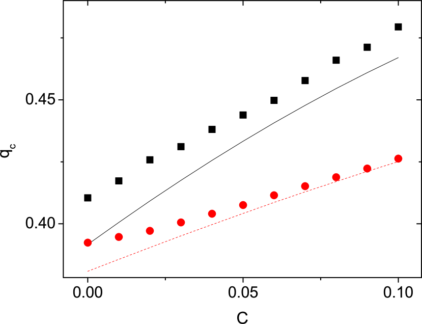
Figure 6: (Color online) Percolation thresholds of slightly clustered networks with truncated degree distribution $P(k)\sim k^{-\lambda}e^{-k/k_{0}}$, $k\geqslant m$. Squares: $\lambda=3$, $m=2$, $k_{0}=10$; Circles: $\lambda=6$, $m=3$, $k_{0}=\infty$. The network size is $10^{6}$, and each data is averaged over 1000 realizations. Solid and dashed lines: theoretical result of Eq. (2) for $\lambda=3$ and $\lambda=6$ respectively.

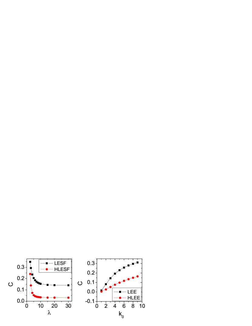
Figure 7: (Color online) Clustering coefficients of the normal (squares) and hollow (circles) networks with scale-free (left panel) and exponential (right panel) degree distributions.

Although Eq. (2) holds only for the case of small clustering coefficient $C$, the analysis above indicates that for large $C$, or if the network has higher order cycles, the fraction of edges that inter-connect existed nodes in a local cluster will further increase. Thus the number of efficient edges connecting to “new” nodes (in comparison to the nodes within the local cluster) may be even smaller, which results in a higher percolation threshold. Thus when a network is more clustered, or has more cycles—not only of order $3$—it will be less robust.

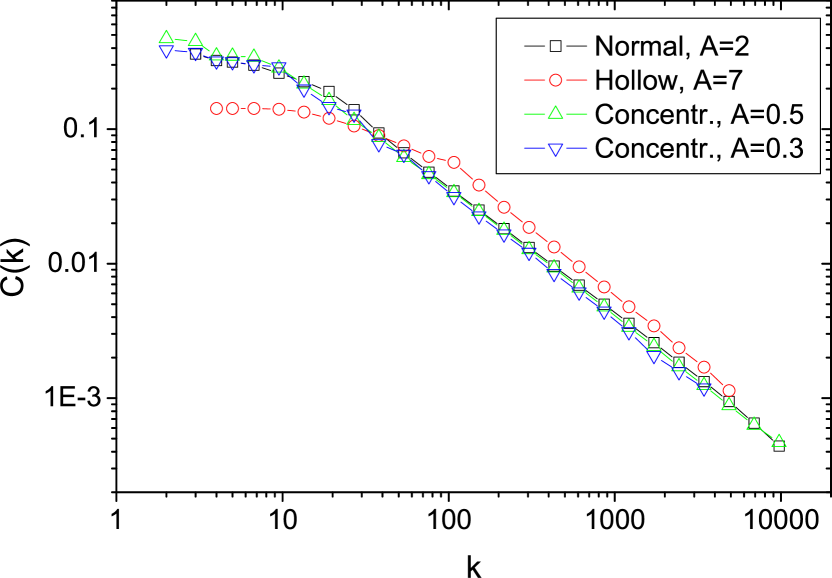
Figure 8: (Color online) Clustering coefficient spectrum for the normal model (squares), hollow model (circles), concentrated model with $A=0.5$ (up triangles), and concentrated model with $A=0.3$ (down triangles). The networks are scale-free with $\lambda=3.0$. The data are log-binned.

Equation 1 shows that the most influential cycles on percolation threshold are triangles; further more, for the same number of edges forming cycles, there will be more triangles than higher order cycles. Thus the decrease of the number of triangles (clustering coefficients) in the same kind of networks will be always accompanied with the drop of percolation thresholds. Figure 7 displays the clustering coefficient $C$ for both normal and hollow networks. It can be seen that the hollow networks have much smaller clustering coefficients. Since the percolation threshold also depend on the spectrum of the clustering coefficient (Eq. (2)), we examined the clustering coefficient spectrum for the normal, hollow and concentrated scale-free networks, and the results are shown in Fig. 8. For normal networks, the spectra for $A>2$ are almost the same as that for $A=2$. The spectra for concentrated networks follow the same scaling law as those for normal networks, and the small fluctuations explain the behavior of clustering coefficient in Fig. 5(a). For hollow networks, the local clustering coefficient is much smaller for nodes with small degrees, while it follows the same scaling relation as that for normal networks when degree is large. Thus the influence of the spectrum of clustering coefficients is not crucial. Therefore the decrease in $C$ for hollow networks is consistent with the drop of the percolation thresholds (Figs 1 and 2).

In short, we have studied how the geographical structure affects the percolation behavior of complex networks, and provided analytical understandings by generating function formalism on networks with cycles. Our study gives a general suggestion on constructing more robust real functional networks, such as the Internet, the power grid network, etc., that arrange the edges to connect neighboring nodes as far as possible. Although it may cost a little more, it will stand a much reduced risk in case of node failures. Also, the hollowing strategy could be useful to maintain the global functions of real world networks during some emergencies, such as epidemic occurrences, eruptions of electronical virus, or cascade failures of power stations, etc.

L. Y. thanks the 100 Person Project of the Chinese Academy of Sciences for their support, the Hong Kong Research Grants Council (RGC), the Hong Kong Baptist University Faculty Research Grant (FRG). and K.Y. thanks the Institute of Geology and Geophysics, CAS for their support. The work is supported by the China National Natural Sciences Foundation with Grant No. 49894190 of a major project and the Chinese Academy of Science with Grant No. KZCX1-sw-18 of a major project of knowledge innovation engineering.

References

- (1) R. Albert and A.-L. Barabási, Rev. Mod. Phys. 74, 47 (2002); M. E. J. Newman, SIAM Rev. 45, 167 (2003); S. N. Dorogovtsev and J. F. F. Mendes, Evolution of Networks (Oxford University Press, Oxford, 2003); R. Pastor-Satorras and A. Vespignani, Evolution and Structure of the Internet (Cambridge University Press, Cambridge, 2004).
- (2) A. Vázquez, R. Pastor-Satorras, and A. Vespignani, Phys. Rev. E 65, 066130 (2002).
- (3) C. von Ferber, Yu. Holovatch, and V. Palchykov, Condens. Matter Phys. 8, 225 (2005); P. Sen, S. Dasgupta, A. Chatterjee, P. A. Sreeram, G. Mukherjee, and S. S. Manna, Phys. Rev. E 67, 036106 (2003).
- (4) W. Li and X. Cai, Phys. Rev. E 69, 046106 (2003); R. Guimerà, S. Mossa, A. Turtschi, and L. A. N. Amaral, Proc. Natl. Acad. Sci. U.S.A. 102 7794 (2005); L. Dall’Asta, A. Barrat, M. Barthelemy and A. Vespignani, J. Statistical Mechanics, P04006 (2006).
- (5) B. J. Gluckman, T. I. Netoff, E. J. Neel, W. L. Ditto, M. L. Spano, and S. J. Schiff, Phys. Rev. Lett. 77, 4098 (1996).
- (6) A. Barrat, M. Barthélemy, R. Pastor-Satorras, and A. Vespignani, Proc. Natl. Acad. Sci. U.S.A. 101 3747 (2004).
- (7) A. F. Rozenfeld, R. Cohen, D. ben-Avraham, and S. Havlin, Phys. Rev. Lett. 89, 218701 (2002); D. ben-Avraham, A. F. Rozenfeld, R. Cohen and S. Havlin, Physica A 330, 107 (2003).
- (8) C. P. Warren, L. M. Sander, and I. M. Sokolov, Phys. Rev. E 66, 056105 (2002).
- (9) P. Sen and S. S. Manna, Phys. Rev. E 68, 26104 (2003); R. Xulvi-Brunet and I. M. Sokolov, Phys. Rev. E 66, 026118 (2002); J. Dall and M. Christensen, Phys. Rev. E 66, 016121 (2002); G. Nemeth and G. Vattay, Phys. Rev. E 67, 036110 (2003); C. Herrmann, M. Barthélemy, P. Provero, Phys. Rev. E 68, 26128 (2003).
- (10) K. Yang, L. Huang and L. Yang, Phys. Rev. E 70, 015102(R) (2004).
- (11) L. Huang, L. Yang, and K. Yang, Phys. Rev. E 73, 036102 (2006).
- (12) A. K. Gupta and A. K. Sen, Physica A, 215, 1 (1995).
- (13) M. E. J. Newman and R. M. Ziff, Phys. Rev. Lett. 85, 4104 (2000); Phys. Rev. E 64, 016706 (2001).
- (14) M. E. J. Newman, I. Jensen, and R. M. Ziff, Phys. Rev. E 65, 021904 (2002).
- (15) P. Holme, B. J. Kim, C. N. Yoon, and S. K. Han, Phys. Rev. E 65, 056109 (2002); A. E. Motter, T. Nishikawa and Y.-C. Lai, Phys. Rev. E 66, 065103(R) (2002); B. K. Singh and N. Gupte, Phys. Rev. E 68, 066121 (2003).
- (16) C. Moore and M. E. J. Newman, Phys. Rev. E 61, 5678 (2000); Phys. Rev. E 62, 7059 (2000).
- (17) R. Cohen, K. Erez, D. ben-Avraham, and S. Havlin, Phys. Rev. Lett. 85, 4626 (2000).
- (18) D. S. Callaway, M. E. J. Newman, S. H. Strogatz, and D. J. Watts, Phys. Rev. Lett. 85, 5468 (2000).
- (19) M. E. J. Newman, S. H. Strogatz, and D. J. Watts, Phys. Rev. E 64, 026118 (2001).
- (20) S. N. Dorogovtsev, A. V. Goltsev, J. F. F. Mendes, Phys. Rev. E 65, 066122 (2002); E. Ravasz and A.-L. Barabási, Phys. Rev. E 67, 26112 (2003); G. Szabo, M. Alava, and J. Kertesz, Phys. Rev. E 67, 56102 (2003).
- (21) S. Maslov and K. Sneppen, Science 296, 910 (2002); B. J. Kim, Phys. Rev. E 69, 045101(R) (2004).