The effect of the range of interaction on the phase diagram of a globular protein

Abstract

Thermodynamic perturbation theory is applied to the model of globular proteins studied by ten Wolde and Frenkel (Science 277, pg. 1976) using computer simulation. It is found that the reported phase diagrams are accurately reproduced. The calculations show how the phase diagram can be tuned as a function of the lengthscale of the potential.

I Introduction

One of the most important problems in biophysics is the characterization of the structure of proteins. The experimental determination of protein structure by means of x-ray diffraction requires that the proteins be prepared as good quality crystals which turns out to be difficult to achieve. Given the fact that recent years have seen an explosion in the number of proteins which have been isolated, the need is therefore greater than ever for efficient methods to produce such crystals. Without finely tuned experimental conditions, often discovered through laborious trial and error, crystallization may not occur on laboratory time-scales or amorphous, rather than crystalline, structures may form. The recent observation by ten Wolde and FrenkeltWF of enhanced nucleation of a model protein in the vicinity of a metastable critical point is thus of great interest and could lead to more efficient means of crystallization if such conditions can be easily identified for a given protein.

Wilson noted that favorable conditions for crystallization are correlated with the behavior of the osmotic second virial coefficientGeorgeWilson and, hence, depend sensitively on temperature. If the second virial coefficient is too large, crystallization occurs slowly and if it is too small, amorphous solids form. By comparing the experimentally determined precipitation boundaries for several different globular proteins as a function of interaction range, controlled by means of the background ionic strength, Rosenbaum et al have shown that the phase diagrams of a large class of globular proteins can be mapped onto those of simple fluids interacting via central force potentials consisting of hard cores and short-ranged attractive tailsRosenbaum1 ,Rosenbaum2 . They also discuss the important fact that the range of interaction can be tuned by varying the composition of the solvents used. The attraction must, in general, be very short ranged if this model is to apply since a fluid-fluid phase transition is not typically observe experimentallyRosenbaum2 and it is known that this transition is only suppressed in simple fluids when the attractions are very short rangedFrenkelYukawa . These studies therefore support the conclusion that the study of simple fluids interacting via potentials with short-ranged attractive tails can give insight into nucleation of the crystalline phase of a large class of globular proteins. ten Wolde and Frenkel have studied nucleation of a particular model globular protein consisting of a hard-core and a modified Lennard-Jones tail by direct free energy measurements obtained from computer simulationstWF . They found that the nucleation rate of a stable FCC solid phase could be significantly enhanced in the vicinity of a metastable critical point. The enhancement is due to the possibility that a density fluctuation in the vapor phase is able to first nucleate a metastable droplet of denser fluid which, in turn, forms a crystal nucleus. The fact that intermediate metastable states can accelerate barrier crossing has been confirmed using kinetic modelsNicolis1 and the physics of the proposed non-classical nucleation model has also been confirmed by theoretical studies based on density functional modelsOxtobyProtein ,GuntonProtein . This observation opens up the possibility of efficiently producing good quality protein crystals provided that it is understood how to tune the interactions governing a given protein so that its phase diagram possesses such a metastable state under experimentally accessible conditions. A prerequisite for achieving this is to go beyond the heavily parameterized studies conducted so far and to be able to accurately predict phase diagrams given knowledge of the range of the protein interactions. In this paper, we describe the application of thermodynamic perturbation theory to calculate the phase diagram based solely on the interaction model. In so far as the range of interaction is important, and not the detailed functional forms, this approach, if successful, gives a direct connection between the phase diagram and the range of interaction without the need for further, phenomenological parameterizations. We show that the theory can be used to successfully reproduce the phase diagrams of ten Wolde and Frenkel based only on the interaction potential and assess the effect of the range of the interatomic potential on the structure of the phase diagram.

In the next Section, the formalism used in our calculations is outlined. This involves the standard Weeks-Chandler-Andersen perturbation theory with modifications to improve its accuracy at high densities. The third Section discusses the application of the perturbation theory to the ten Wolde-Frenkel interaction model. Whether or not perturbation theory is applicable to this type of system is not immediately evident: the hard-core square well potential has long served as a test case for developments in perturbation theoryBarkerHend_WhatIsLiquid . So we show how the size of the various contributions to the total free energy varies with temperature and that second order contributions to the free energy are of negligible importance. In the fourth Section, the calculated phase diagram for the hard core plus modified Lennard-Jones tail is shown to be in good agreement with the reported Monte Carlo (MC) results. Since the perturbation theory is also well knownRee2 to give a good description of long-ranged potentials such as the standard Lennard-Jones, we expect that it can be used with some confidence to explore the effect of the length scale of the potential on the phase behavior of the systems. To illustrate, we present the phase diagram as a function of the range of the modified Lennard-Jones tail and show that the appearance of the metastable state requires only a minor modification of the range of the potential. The final Section contains our conclusions where we discuss the prospect for using the perturbation theory free energy function as the basis for density functional studies of the nucleation process and for studies of the effect of fluctuations on the nucleation rate.

II Thermodynamic perturbation theory

Thermodynamic perturbation theory allows one to express the Helmholtz free energy $F$ of a system in terms of a perturbative expansion about some reference system. There are a number of different approaches to constructing the perturbative expansions such as the well known Weeks-Chandler-Andersen (WCA)WCA1 ,WCA2 ,WCA3 ,HansenMcdonald theory and the more recent Mansoori-Canfield/Rasaiah-Stell theoryStell2004 . The latter appears to be more accurate for systems with soft repulsions at small separations while the former works better for systems with stronger repulsions. Here, we will be interested in a hard-core potential with a modified Lennard-Jones tail, so we use the WCA theory as modified by Ree and coworkersRee1 ,Ree2 ,ReeSol as discussed below. The first step is to divide the potential into a (mostly) repulsive short-ranged part and a longer ranged (mostly) attractive tail according to the prescription

$$v(r) = v_{0}\left(r\right)+w\left(r\right)$$ (1)

$$v_{0}\left(r\right) = \left\{\begin{array}[]{c}v\left(r\right)-v\left(r_{0}\right)-v^{\prime}\left(r_{0}\right)\left(r-r_{0}\right),\;r<r_{0}\\ 0,\;r>r_{0}\end{array}\right.$$ (4)

$$w\left(r\right) = \left\{\begin{array}[]{c}v\left(r_{0}\right)+v^{\prime}\left(r_{0}\right)\left(r-r_{0}\right),\;r<r_{0}\\ v\left(r\right),\;r>r_{0}\end{array}\right..$$ (7)

The short ranged part is generally repulsive and can therefore be well approximated by a hard-sphere reference system. The long-ranged tail describes the attractive forces and must also be accounted for so that distinct liquid and gas phases exist (i.e. so that the phase diagram exhibits a Van der Waals loop). There are a number of versions of the WCA-type perturbation theory depending on the choice of the separation point $r_{0}$. Barker and HendersonBarkerHend chose the separation point $r_{0}$ to be the point at which the potential goes to zero, $v\left(r_{0}\right)=0$, (they also did not include the linear term in the expressions above). Subsequently, WCA achieved a better description of the Lennard-Jones phase diagram by taking the separation point to be at the minimum of the potential, $v^{\prime}\left(r_{0}\right)=0$ . ReeRee1 first suggested that the free energy be minimized with respect to $r_{0},$ and introduced the linear terms in eq.(1), in which case the first-order perturbation theory is equivalent to a variational theory based on the Gibbs-Bugolyubov inequalitiesHansenMcdonald . Later, Ree and coworkers showed that essentially the same results could be achieved with the prescription

$$r_{0}=\min\left(r_{\min},r_{nn}\right)$$ (8)

where $r_{\min}$ is the minimum of the potential, $v^{\prime}\left(r_{\min}\right)=0$ and $r_{nn}=2^{\frac{1}{6}}\rho^{-1/3}$, where $\rho$ is the density, is the FCC nearest-neighbor distanceRee2 . For low densities, this amounts to the original WCA prescription whereas for higher densities, the separation point decreases with increasing density. In this case, the linear term in the definition of $v_{0}\left(r\right)$ ensures the continuity of the first derivative of the potential. Calculations for the Lennard-Jones potential, as well as inverse power potentials, show that this modification of the original WCA theory gives improved results at high density. Finally, eq.(8) was modified to switch smoothly from $r_{\min}$ to $r_{nn}$ as the density increases so as to avoid discontinuities in the free energy as a function of density and thus singularities in the pressureReeSol . Below, we will refer to this final form of the Weeks-Chandler-Andersen-Ree theory as the WCAR theory.

II.1 Contribution of the long-ranged part or the potential

The contribution of the long-ranged part of the potential to the free energy is handled perturbatively in the so-called high-temperature expansionHansenMcdonald

$$\frac{1}{N}\beta F-\frac{1}{N}\beta F_{0}=\frac{1}{N}\beta\left\langle W\right\rangle_{0}+\frac{1}{2N}\beta^{2}\left[\left\langle W^{2}\right\rangle_{0}-\left\langle W\right\rangle_{0}^{2}\right]+...$$ (9)

where $F_{0}$ is the free energy of a system of $N$ particles subject only to the short-ranged potential $v_{0}\left(r\right)$ at inverse temperature $\beta=1/k_{B}T$ and where the total attractive energy is

$$W=\sum_{1\leq i<j\leq N}w\left(r_{ij}\right).$$ (10)

The brackets $\left\langle...\right\rangle_{0}$ indicate an equilibrium average over a system interacting with the potential $v_{0}$. The first term on the right is easily calculated since it only involves the pair distribution function of the reference system

$$\frac{1}{N}\beta\left\langle W\right\rangle_{0}=\frac{1}{2}\beta\rho\int d\overrightarrow{r}\;g_{0}\left(r\right)w\left(r\right)$$ (11)

where $g_{0}\left(r\right)$ is the pair distribution function of the reference system. The second term requires knowledge of three- and four-body correlations for which good approximations are not available. Its value is typically estimated using Barker and Henderson’s ”macroscopic compressibility” approximationBHMacroscopicCompressibility ,BarkerHend_WhatIsLiquid

$$\frac{1}{2N}\beta^{2}\left[\left\langle W^{2}\right\rangle_{0}-\left\langle W\right\rangle_{0}^{2}\right]\simeq-\frac{1}{4}\beta^{2}\rho\left(\frac{\partial\rho}{\partial\beta P_{0}}\right)\int d\overrightarrow{r}\;g_{0}\left(r\right)w^{2}\left(r\right)$$ (12)

where $P_{0}$ is the pressure of the reference system at temperature $k_{B}T=1/\beta$ and density $\rho$.

II.2 Contribution of the short-ranged part of the potential

The description of the reference system is again accomplished by perturbation theory. Since the potential $v_{0}\left(r\right)$ is not very different from a hard core potential, this perturbation theory does not involve the high temperature expansion but, rather, involves a functional expansion in the quantity $\exp\left(-\beta v_{0}\left(r\right)\right)-\exp\left(-\beta v_{hs}\left(r;d\right)\right)$ where $v_{hs}\left(r;d\right)$ is the hard sphere potential for a hard-sphere diameter $d$. The result is

$$\frac{1}{N}\beta F_{0}-\frac{1}{N}\beta F_{hs}\left(\rho d^{3}\right)=\int d\overrightarrow{r}\;y_{hs}\left(r\right)\left(\exp\left(-\beta v_{0}\left(r\right)\right)-\exp\left(-\beta v_{hs}\left(r;d\right)\right)\right)+...$$ (13)

where $y_{hs}\left(r,\rho d^{3}\right)$ is the hard-sphere cavity function, related to the pair distribution function through $g_{hs}(r)=\exp\left(-\beta v_{hs}\left(r;d\right)\right)y_{hs}(r)$. Several methods of choosing the hard-sphere diameter of the reference system are common. The WCA prescription is to force the first order term to vanish

$$0=\int d\overrightarrow{r}\;y_{hs}\left(r\right)\left(\exp\left(-\beta v_{0}\left(r\right)\right)-\exp\left(-\beta v_{hs}\left(r;d\right)\right)\right).$$ (14)

and a simple expansion about $r=d$ gives the cruder Barker and Henderson approximationHansenMcdonald which gives

$$\int dr\left(\exp\left(-\beta v_{0}\left(r\right)\right)-1\right)+\int dr\left(1-\exp\left(-\beta v_{hs}\left(r;d\right)\right)\right)\simeq 0.$$ (15)

In either case, one can then consistently approximate the pair distribution function of the reference state as either

$$g_{0}\left(r\right)\simeq g_{hs}\left(r\right)$$ (16)

or

$$g_{0}\left(r\right)\simeq\exp\left(-\beta v_{0}\left(r\right)\right)y_{hs}\left(r\right)$$ (17)

where the difference between using one expression or the other is of the same size as neglected terms in the perturbation theory. Here, we follow Ree et alRee2 in using the WCA prescription for the hard-sphere diameter, eq.(14) and the first approximation, eq.(16), for the pair distribution function. Then, the complete expression for the free energy becomes

$$\frac{1}{N}\beta F = \frac{1}{N}\beta F_{hs}\left(\rho d^{3}\right)+\int d\overrightarrow{r}\;y_{hs}\left(r\right)\left(\exp\left(-\beta v_{0}\left(r\right)\right)-\exp\left(-\beta v_{hs}\left(r;d\right)\right)\right)$$

$$+\frac{1}{2}\beta\rho\int d\overrightarrow{r}\;g_{hs}\left(r\right)w\left(r\right)$$

$$-\frac{1}{4}\beta\rho\left(\frac{\partial\rho}{\partial P_{0}}\right)\int d\overrightarrow{r}\;g_{hs}\left(r\right)w^{2}\left(r\right).$$

The pressure, $P$, and chemical potential $\mu$ are calculated from the free energy using the standard thermodynamic relations

$$\frac{\beta P}{\rho} = \rho\frac{\partial}{\partial\rho}\frac{1}{N}\beta F$$ (19)

$$\beta\mu = \frac{1}{N}\beta F+\frac{\beta P}{\rho}.$$

II.3 Description of the reference liquid

The calculation of liquid phase free energies require as input the properties of the hard sphere liquid. These are known to a high degree of accuracy and introduce no significant uncertainty, nor any new parameters, into the calculations.

The properties of low density hard-sphere liquids are well described by the Percus-Yevick (PY) approximation but this is not adequate for the dense liquids to be considered here. So for the hard sphere cavity function, we have used the model of Henderson and GrundkeHendGrundke which modifies the PY description so as to more accurately describe dense liquids. The corresponding pair distribution function is then that of Verlet and WeissVWgr and the equation of state, as obtained from it by both the compressibility equation and the pressure equation, is the Carnahan-Starling equation of stateHansenMcdonald . The free energy as a function of density follows immediately and is given by

$$\frac{1}{N}\beta F_{hs}\left(\rho d^{3}\right)=\ln\left(\rho\Lambda^{3}\right)-1+\eta\frac{4-3\eta}{\left(1-\eta\right)^{2}}$$ (20)

where $\eta=\rho d^{3}$. The second term of eq.(II.2) is easily evaluated numerically as its kernel is sharply peaked about $r=d$ . The most troublesome part of the calculation is the evaluation of the contributions of the long-ranged part of the potential, $w\left(r\right)$ . One method is to divide the necessary integrals along the lines

$$\int d\overrightarrow{r}\;g_{hs}\left(r\right)w\left(r\right)=\int d\overrightarrow{r}\;w\left(r\right)+\int d\overrightarrow{r}\;\left(g_{hs}\left(r\right)-1\right)w\left(r\right)$$ (21)

where the first piece can be calculated analytically and the second involves the structure function $g_{hs}\left(r\right)-1$ which is relatively short ranged allowing a numerical evaluation. However, at high densities this can still be difficult to evaluate as the hard-sphere structure extends for considerable distances. In the Appendix, we discuss a more efficient method of evaluation based on Laplace transform techniques. We have used both methods and obtained consistent results: in general, the second is much easier to implement and numerically more stable.

II.4 Description of the reference solid

To calculate the properties of the solid phase, the same expressions are used except that the reference free energy is now that of the hard-sphere solid and the pair distribution function is the spherical average of the hard-sphere pair distribution function. Both of these quantities can be obtained by means of classical density functional theory, but here we choose the simpler, and older, approach which makes use of analytic fits to the results of computer simulations together with the known high-density limit of the equation of state. This limits the present calculations to the investigation of the FCC solid phase as this is the only one for which extensive simulations have been performed. We stress that these fits are very good and that they introduce no new parameters into the calculations of the phase diagrams.

In the calculations presented below, we have used the equation of state proposed by HallHallHsSolidEOS

$$\frac{\beta P}{\rho} = 3\frac{\eta}{\eta_{c}-\eta}+2.557696+0.1253077b+0.1762393b^{2}-1.053308b^{3}$$

$$+2.818621b^{4}-2.921934b^{5}+1.118413b^{6}$$

$$b = 4\left(1-\frac{\eta}{\eta_{c}}\right)$$

where $\eta_{c}=\frac{\pi}{6}\sqrt{2}$ is the value of the packing fraction at close packing. Notice that the first term is the high density limit of the Lennard-Jones-Devonshire cell theory which is expected to be exact near close packing (see, e.g., the discussion in AlderHsSolidEOS ). The free energy is then calculated by integrating from the desired density to the close-packing density giving

$$\beta F=\beta F_{0}-\int_{\eta}^{\eta_{c}}\left[\frac{\beta P}{\rho}-\left(\frac{\beta P}{\rho}\right)_{LJD}\right]\frac{d\eta}{\eta}.$$ (23)

For the spherically-averaged pair distribution function for the FCC solid, we use the analytic fits of Kincaid and WeissWKSolidGr

$$g_{KW}\left(r\right)=\left(A/x\right)\exp\left[-w_{1}^{2}\left(x-x_{1}\right)-w_{2}^{4}\left(x-x_{1}\right)^{4}\right]+\frac{w}{24\eta\sqrt{\pi}}\sum_{i=2}^{\infty}\frac{n_{i}}{x_{i}x}\exp\left(-w^{2}\left(x-x_{1}\right)^{2}\right).$$ (24)

Here $x=r/d$, the parameter $A$ is fixed by requiring that the pressure equation reproduce the Hall equation of state

$$\left(\frac{\beta P}{\rho}\right)_{Hall}=1+4\eta g_{KW}\left(1\right),$$ (25)

and the parameters $w_{1},$ $w_{2}$ and $w$ are given as functions of density by analytic fits to the MC dataWKSolidGr . No such fit is given for the parameter $x_{1}$ so its value must be determined by interpolating from the values extracted from the MC data as given in WKSolidGr . The quantities $n_{i}$ and $x_{i}$ are the number of neighbors and the position of the $i$-th lattice shell respectively. Note that Ree et al suggest using the earlier parameterization of WeisWeissSolidGr at lower densities, where it is slightly more accurate, and the Kincaid-Weis version at higher densities. We have not done this because it leads to discontinuities in the free energy as a function of density at the point the switch is made. Since these are just empirical fits, we do not believe there is a significant loss of accuracy.

III Application to a model protein intermolecular potential

III.1 The potential

The only input needed for the perturbative calculation outlined in Section II is the intermolecular potential: there are no phenomenological parameters to specify. The goal of this work is to show how to construct a realistic free energy functional with which to study nucleation of protein crystallization using the model potential of ten Wolde and FrenkeltWF . This interaction model consists of a hard-sphere pair potential with an attractive tail

$$v\left(r\right)=\left\{\begin{array}[]{c}\infty\;,\;r<\sigma\\ \frac{4\varepsilon}{\alpha^{2}}\left[\frac{1}{\left(\left(\frac{r}{\sigma}\right)^{2}-1\right)^{6}}-\alpha\frac{1}{\left(\left(\frac{r}{\sigma}\right)^{2}-1\right)^{3}}\right]\;,\;r>\sigma\end{array}\right.$$ (26)

The tail is actually a modified Lennard-Jones potential and the two are related by

$$\Theta\left(r-\sigma\right)v\left(r\right)=\Theta\left(r-\sigma\right)v_{LJ}\left(\alpha^{1/6}\sigma\sqrt{\left(\frac{r}{\sigma}\right)^{2}-1}\right).$$ (27)

As such, the potential decays as a power law and is not short-ranged in the usual sense. Nevertheless, as $\alpha$ becomes larger, the range of the potential decreases: for example, the minimum of the potential is

$$\frac{r_{\min}}{\sigma} = \sqrt{1+\left(\frac{2}{\alpha}\right)^{1/3}}$$ (28)

$$v\left(r_{\min}\right) = -\varepsilon.$$

which approaches the hard core for large $\alpha$ . Furthermore, for a fixed position $r>r_{\min}$, the value of the potential decreases with increasing $\alpha$ relative to its minimum. For example,

$$v\left(2\sigma\right)/v\left(r_{\min}\right)=\frac{108\alpha-4}{729\alpha^{2}}$$ (29)

so that as $\alpha$ increases, the interactions of particles separated by much more than $r_{\min}$ contribute less and less to the total energy compared to the contribution of particles that are close together. Figure 1 shows the evolution of the shape of the potential as $\alpha$ increases. The range of the potential varies from about $2.5$ hard sphere diameters for $\alpha=1$ to less than $1.25$ diameters for $\alpha=50$. Also shown in the figure is the separation of the potential into long- and short-ranged pieces for the case $\alpha=50$ where it is clear that even for this very short-ranged potential, the long-ranged function $W(r)$ varies relatively slowly compared to the short-ranged repulsive potential $V_{0}\left(r\right)$.

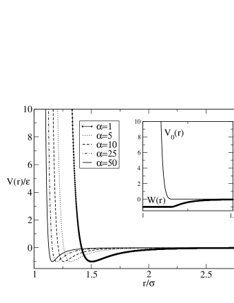
Figure 1: The ten Wolde-Frekel potential as a function of $\alpha$. The inset shows the division of the potential into long-ranged and short-ranged parts for $\alpha=50$.

III.2 Comparison of various approximations

Figure 2 shows the contributions of the various terms contributing to the free energy at two temperatures. In both cases, the second order term is seen to be negligible. This is because at low density, the free energy is dominated by the ideal-gas contribution, all other contributions going to zero with the density, whereas at moderate to high density, the compressibility controlling the size of the contribution of the second order term, see eq.(II.2), diminishes quickly from its zero density limit of $1.0$ to something on the order of $0.1$ at moderate densities and is of order $0.01$ at high densities. We conclude that the second order contributions, at least calculated within the macroscopic compressibility approximation, eq.(12), can be neglected.

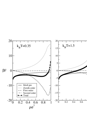
Figure 2: The various terms contributing to the total free energy as a function of density for two different temperatures. At the lower temperature, the first order contribution dominates the hard-sphere contribution whereas at higher temperatures, the zeroth order terms dominate.

In the case of the lower temperature, $k_{B}T/\varepsilon=0.35$, the first order contributions quickly grow with density until at high densities, they are larger than the zeroth order contributions thus suggesting that the perturbation theory will not prove very accurate. At the higher temperature, $k_{B}T/\varepsilon=1.5$, the first order contributions are much better controlled and we expect the perturbation theory to be relatively accurate.

We have also tested the various approaches to the selection of the separation point of the potential - the WCA prescription, eq.(8), the WCAR prescription and minimization of the free energy with respect to $r_{0}$. As expected, the only significant differences occur at high density, where variations of the free energy of 10% occur, but we find virtually no effect on the phase diagram.

IV Phase diagrams

Figure 3 shows the phase diagram as calculated from the WCAR theory for the potential and parameters used by ten Wolde and FrenkeltWF and its comparison to the results of Monte Carlo simulations by these authors for $\alpha=50$. The lines, from our calculations, and the symbols, from the simulations, divide the density-temperature phase diagram into three parts: the liquid region (low density and high temperature), the fluid-solid coexistence region and the solid region (at high density). In the calculations, the lines are determined by finding, for a given temperature, the liquid and solid densities that give equal pressures and chemical potentials for the two phases as determined using eq.(19) based on the liquid and solid free energy calculations (which differ only in the equation of state and pair distribution function of the reference states). The fluid-fluid coexistence is determined similarly except that the free energy for both phases is calculated using the same reference state (the hard-sphere fluid) with the resulting free energy exhibiting a Van der Waals loop.

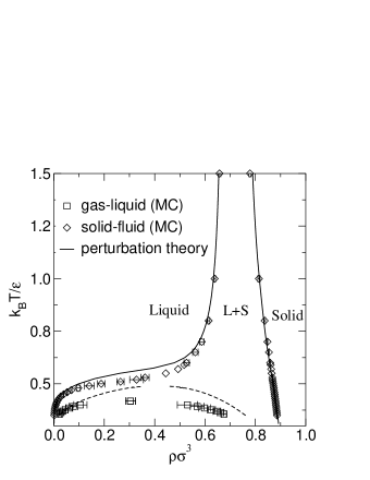
Figure 3: Comparison of the predicted phase diagram, lines, to the Monte Carlo results, symbols, of ref.tWF for $\alpha=50$. Some error bars are superposed on the symbols.

The calculations and simulations are in good qualitative agreement with a fluid-fluid critical point that is suppressed by the fluid-solid phase boundaries. The values of the coexisting densities are in good agreement at low temperatures, where the liquid density is very low and at high temperatures. That these limits agree is as expected from our discussion of the relative sizes of the various contributions to the free energy. It is perhaps surprising that the agreement is so good even for temperatures as low as $k_{B}T/\varepsilon\sim 1$. The intermediate temperature values, where the attractive tail and finite density effects are important, are the most poorly described. The same is true of the fluid-fluid coexistence curve. The critical point is estimated to occur at about $k_{B}T/\varepsilon\sim 0.48$ and $\rho\sigma^{3}\sim 0.4$ whereas the simulation results are $k_{B}T/\varepsilon\sim 0.4$ and $\rho\sigma^{3}\sim 0.3$. We have tested these results by using different choices for the pair distribution function of the reference state (see eqs.(16)-(17)), and different choices for the division of the potential (such as minimizing the free energy with respect to the break point) but none of these alternatives produces any significant change.

An interesting feature of short-ranged interactions is that under some circumstances, they give rise to solid-solid transitions where the lattice structure remains the same but solids of different densities can coexist (i.e. a van der Waals loop occurs in the solid free energy)BausSolidSolid . We have searched for, but find no evidence of, such a transition with the present potential.

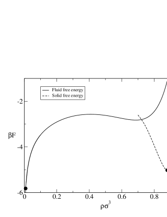
Figure 4: Calculated free energies as a function of density for the liquid and solid phases at $k_{B}T/\epsilon=0.4$ and for $\alpha=50$.The points mark the location of the coexisting phases.

To give some idea of the typical energy barrier between the coexisting phases, we show in Fig. 4 the calculated isothermal free energies as a function of density between the coexisting fluid and solid phases at $k_{B}T/\epsilon=0.4$ for the short-ranged ($\alpha=50$) potential. The fluid has a density of 0.008 and Helmholtz free energy of -5.82 in reduced units. The maximum free energy is -2.57 and the solid free energy is -5.02 at a density of 0.88.

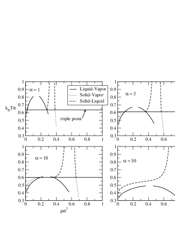
Figure 5: Calculated phase diagrams as a function of $\alpha$ showing that the critical point is suppressed for $\alpha\geq 10$.

Figure 5 shows the phase diagrams calculated from the WCAR theory as a function of the range of the potential (i.e., different values of $\alpha$). For $\alpha=1$, for which the minimum of the potential well is $r_{min}=1.5$ and corresponding to a tail that closely resembles a standard Lennard-Jones interaction, the phase diagram has the classical form exhibiting three stable phases, a critical point and a triple point. As $\alpha$ increases, and the range of the potential decreases, the critical point moves towards the triple point. Even for $\alpha=5$ and $r_{min}=1.31$, the critical point lies very near the triple point and the two become nearly identical for $\alpha=10$ and $r_{min}=1.26$. Our conclusion is that for this model, the suppression of the triple point occurs when the range of the potential, as characterized by its minimum, falls to about a quarter of the hard-core diameter.

V Conclusions

Our aim here has been to provide a fundamental model of protein crystallization without the need for parameterizations other than the interaction potential. Since the potential for globular proteins can be tuned, by varying e.g. the background ionic strength of the solutions, this provides a rather direct connection between theoretical indications of favorable conditions for nucleation and experimentally accessible control parameters.

We have shown that thermodynamic perturbation theory gives a good, semi-quantitative estimate of the phase diagram of a model interaction for globular proteins. The accuracy of the perturbation theory is expected to improve as the range of the potential increases so, e.g., the prediction of the value of $\alpha$ at which the critical point becomes suppressed is expected to be reasonably accurate. Unlike the results of a recent study of colloids interacting via short-ranged potentialsHansenPert , we do not find that the second order terms in the high-temperature expansion play an important role in the structure of the phase diagram.

This free energy calculation, which only uses the interaction model as input, should be contrasted with other more phenomenological approaches. In phase field models, the free energy is taken to be a function of one or more order parameters. The actual form of the free energy is typically of the Landau form which is to say, a square-gradient term plus an algebraic function of more than second order in the order parameter. The coefficients of these terms must be fitted to experimental data and the adequacy of the assumed function is difficult to assess. Similarly, the recent density functional models of TalanquerOxtobyProtein and ShiryayevGuntonProtein depend on an ad hoc free energy functional, based on the van der Waals free energy model for the fluid, with several phenomenological parameters.

We believe that our work can serve as the basis for further theoretical study of the nucleation of globular proteins using density functional theory. While the present description of the two phases requires as input separate equations of state and pair distribution functions for the reference hard sphere fluid and solid phases, standard methods exist for interpolating between these so as to provide a single, unified free energy functional suitable to the study of free energy barriers (see,e.g. ref.OLW ). Such a unified model can be used to study static properties, such as the structure of the critical nucleas, using density functional theory as well as the effect of fluctuations on the transition rates by the addition of noise obeying the fluctuation-dissipation theorem.

Finally, it would be desirable to confront the approach developed here to experiments aiming to determine the interaction potential and the phase diagram of concrete globular proteins of interest such as lysozyme and catalase. In recent years, considerable effort was devoted to protein crystallization under microgravity conditions on the grounds that some undesirable effects such as density gradients and advection present in earth-bound experiments can be virtually suppressedGarciaRuiz . In parallel, earth-bound experiments are being carried out to determine conditions and parameters to be used in a microgravity experiment. In either case, the role of the metastable critical point has so far not been addressed in a detailed manner. We believe that the availability of a theory as parameter-free as possible like the one developed in the present work could provide the frame for undertaking such a study on a rational basis.

Appendix A Evaluation of long-ranged contribution to the free energy

We begin by writing the first order contribution of the long-ranged potential as

$$\int d\overrightarrow{r}\;g_{hs}\left(r\right)w\left(r\right)=\int d\overrightarrow{r}\;g_{hs}\left(r\right)v\left(r\right)-\int d\overrightarrow{r}\;g_{hs}\left(r\right)v_{0}\left(r\right)$$ (30)

so that the second term involves the very short ranged function $v_{0}\left(r\right)$ and is easily performed numerically. Our focus is therefore on the evaluation of the first term on the right. If we write the potential as the sum of a hard-core and a continuous tail

$$v\left(r\right)=v_{hs}\left(r\right)+\Theta\left(r-\sigma\right)v_{tail}\left(r\right)$$ (31)

and the effective hard-sphere diameter $d$ $\geq$ $\sigma$, as it clearly will always be, then

$$\int d\overrightarrow{r}\;g_{hs}\left(r\right)v\left(r\right) = \int d\overrightarrow{r}\;\Theta\left(r-d\right)y_{hs}\left(r\right)v\left(r\right)$$

$$= \int d\overrightarrow{r}\;\Theta\left(r-d\right)y_{hs}\left(r\right)v_{tail}\left(r\right)$$

$$= \int d\overrightarrow{r}\;g_{hs}\left(r\right)v_{tail}\left(r\right)$$

so that we can ignore the discontinuity of the hard-core potential and treat and simply deal with the continuous tail potential. The first term can be evaluated by introducing the inverse Laplace transform of $rv_{tail}\left(r\right)$ ,

$$rv_{tail}\left(r\right)=\int_{0}^{\infty}ds\;\exp\left(-sr\right)V_{tail}\left(s\right)$$ (33)

and likewise for $rg_{hs}\left(r\right)$ so that

$$\int d\overrightarrow{r}\;g_{hs}\left(r\right)v_{tail}\left(r\right) = 4\pi\int_{0}^{\infty}dr\;r^{2}g_{hs}\left(r\right)v_{tail}\left(r\right)$$

$$= 4\pi\int_{0}^{\infty}ds\;V_{tail}\left(s\right)\int_{0}^{\infty}dr\;rg_{hs}\left(r\right)\exp\left(-sr\right)$$

$$= 4\pi\int_{0}^{\infty}ds\;V_{tail}\left(s\right)G\left(s\right)$$

where $G(s)$ is the Laplace transform of $rg_{hs}\left(r\right)$, which is known analytic function in the PY approximation

$$G(s;d) = d^{2}G_{PY}(sd)$$ (35)

$$G_{PY}(x) = \frac{x\exp\left(-x\right)F\left(x\right)}{1+12\eta\exp\left(-x\right)F\left(x\right)}$$

$$F\left(x\right) = -\frac{1}{12\eta}\frac{1+Ax}{1+\left(A-1\right)x+\left(\frac{1}{2}-A\right)x^{2}+\left(\frac{1}{2}A-\frac{1+2\eta}{12\eta}\right)x^{3}}$$

$$A = \frac{1+\eta/2}{1+2\eta}.$$

The integral in eq.(A) is controlled by the exponential decay of $G(s;d)$ and is easily performed numerically. Note that for the ten Wolde-Frenkel potential, we have that

$$V_{tail}\left(s\right)=\frac{\varepsilon}{960\alpha^{2}}\left(\begin{array}[]{c}\left(\left(s\sigma\right)^{5}+45\left(s\sigma\right)^{3}+\left(105+480\alpha\right)s\sigma\right)\sinh s\sigma\\ -\left(10\left(s\sigma\right)^{4}+\left(105+480\alpha\right)\left(s\sigma\right)^{2}\right)\cosh s\sigma\end{array}\right).$$ (36)

The Percus-Yevick pair distribution function becomes exact at low densities but is only semi-quantitatively accurate at moderate to high densities. Compared to the pdf determined from computer simulations, its oscillations are slightly out of phase and the pressure calculated from it is in error. The Verlet Weiss pair distribution function is a semi-empirical modification of the basic Percus-Yevick result designed to correct these flaws. It is written as

$$g_{VW}\left(r;\rho,d\right)=\Theta\left(r-d\right)\left(g_{PY}\left(r;\rho,d_{0}\right)+\frac{C}{r}\exp\left(-m(r-d)\right)\cos\left(m\left(r-d\right)\right)\right)$$ (37)

where the step function $\Theta\left(r-d\right)$ ensures the fundamental property that the pdf vanishes inside the core, $d_{0}$ is an effective hard-sphere diameter which has the effect of shifting the phase of the oscillations, and $C$ and $m$ are chosen to give the accurate Carnahan-Starling equation of state via both the pressure equation and the compressibility equation. To apply the Laplace technique in this case requires some care since what we know is the Laplace transform of $g_{PY}\left(r;\rho,d_{0}\right)$ and not that of $\Theta\left(r-d\right)g_{PY}\left(r;\rho,d_{0}\right)$. So we rewrite eq.(37) as

$$g_{VW}\left(r;\rho,d\right) = g_{PY}\left(r;\rho,d_{0}\right)+\left(\Theta\left(r-d\right)-\Theta\left(r-d_{0}\right)\right)g_{PY}\left(r;\rho,d_{0}\right)$$

$$+\Theta\left(r-d\right)\frac{C}{r}\exp\left(-m(r-d)\right)\cos\left(m\left(r-d\right)\right)$$

thus separating out the known PY contribution. This gives

$$\int d\overrightarrow{r}\;g_{hs}\left(r\right)v_{tail}\left(r\right) = \int d\overrightarrow{r}\;g_{PY}\left(r;\rho,d_{0}\right)v_{tail}\left(r\right)$$

$$+4\pi\int_{d_{0}}^{d}r^{2}dr\;g_{PY}\left(r;\rho,d_{0}\right)v_{tail}\left(r\right)$$

$$+4\pi\int_{d}^{\infty}r^{2}dr\;\frac{C}{r}\exp\left(-m(r-d)\right)\cos\left(m\left(r-d\right)\right)v_{tail}\left(r\right)$$

where the first integral can be evaluated via the Laplace transform technique, provided that $d_{0}\geq\sigma$, the second integral is over a finite interval (for which one could analytically approximate the pair distribution function as in ref.HendGrundke ) while the third integral is easily evaluated numerically. All parts of the calculation are therefore well controlled.

Finally, we note that the same techniques can be adapted to the evaluation of the second order contribution to the free energy.

References

- (1) P. R. ten Wolde and D. Frenkel, Science 77, 1975 (1997).
- (2) A. George and W. W. Wilson, Acta Cryst. D 50, 361 (1994).
- (3) D. F. Rosenbaum and C. F. Zukoski, J. Cryst. Growth 169, 752 (1996).
- (4) D. F. Rosenbaum, P. C. Zamora, and C. F. Zukoski, Phys. Rev. Lett. 76, 150 (1996).
- (5) M. H. J. Hagen and D. Frenkel, J. Chem. Phys. 101, 4093 (1994).
- (6) G. Nicolis and C. Nicolis, Physica A 323, 139 (2003).
- (7) V. Talanquer and D. W. Oxtoby, J. Chem. Phys. 109, 223 (1998).
- (8) A. Shiryayev and J. D. Gunton, J. Chem. Phys. 120, 8318 (2004).
- (9) J. A. Barker and D. Hendersen, Rev. Mod. Phys. 48, 587 (1976).
- (10) H. S. Kang, C. S. Lee, T. Ree, and F. H. Ree, J. Chem. Phys. 82, 414 (1985).
- (11) D. Chandler and J. D. Weeks, Phys. Rev. Lett. 25, 149 (1970).
- (12) D. Chandler, J. D. Weeks, and H. C. Andersen, J. Chem. Phys. 54, 5237 (1971).
- (13) H. C. Andersen, D. Chandler, and J. D. Weeks, Phys. Rev. A 4, 1597 (1971).
- (14) J.-P. Hansen and I. McDonald, Theory of Simple Liquids (Academic Press, San Diego, Ca, 1986).
- (15) D. Ben-Amotz and G. Stell, J. Chem. Phys. 120, 4844 (2004).
- (16) F. H. Ree, J. Chem. Phys. 64, 4601 (1976).
- (17) H. S. Kang, , T. Ree, and F. H. Ree, J. Chem. Phys. 82, 414 (1985).
- (18) J. A. Barker and D. Hendersen, J. Chem. Phys. 47, 4714 (1967).
- (19) J. A. Barker and D. Henderson, J. Chem. Phys. 47, 2856 (1967).
- (20) D. Hendersen and E. W. Grundke, J. Chem. Phys. 63, 601 (1975).
- (21) L. Verlet and J. J. Weis, Phys. Rev. A 5, 939 (1972).
- (22) K. Hall, J. Chem. Phys. 57, 2252 (1972).
- (23) B. J. Alder, W. G. Hooever, and D. A. Young, J. Chem. Phys. 49, 3688 (1968).
- (24) J. M. Kincaid and J. J. Weis, Molecular Physics 34, 931 (1977).
- (25) J.-J. Weis, Molecular Physics 28, 187 (1974).
- (26) C. F. Tejero, A. Daanoun, H. N. W. Lekkerkerker, and M. Baus, Phys. Rev. Lett. 73, 752 (1994).
- (27) B. Rotenberg, J. Dzubiella, J.-P. Hansen, and A. A. Louis, Mol. Phys. 102, 1 (2004).
- (28) R. Ohnesorge, H. Lowen, and H. Wagner, Phys. Rev. A 43, 2870 (1991).
- (29) J. M. Garcia, J. Drenth, M. Reis-Kautt, and A. Tardieu, in A world without gravity - research in space for health and industrial processes, edited by G. Seibert (European Space Agency, Noordwijk, The Netherlands, 2001).