Tumor growth instability and the onset of invasion

Abstract

Motivated by experimental observations, we develop a mathematical model of chemotactically directed tumor growth. We present an analytical study of the model as well as a numerical one. The mathematical analysis shows that: (i) tumor cell proliferation by itself cannot generate the invasive branching behaviour observed experimentally, (ii) heterotype chemotaxis provides an instability mechanism that leads to the onset of tumor invasion and (iii) homotype chemotaxis does not provide such an instability mechanism but enhances the mean speed of the tumor surface. The numerical results not only support the assumptions needed to perform the mathematical analysis but they also provide evidence of (i), (ii) and (iii). Finally, both the analytical study and the numerical work agree with the experimental phenomena.

I Introduction

Experiments have shown that a variety of tumor cells produce both protein growth factors and their corresponding receptors, enabling a mechanism termed autocrine or paracrine, if the stimulus not only affects the source but also its bystander cells ref1 . Such polypeptide growth factors can, for example, stimulate tumor cell growth and invasion, such as in the case of hepatocyte growth factors ref2 and epidermal growth factor ref3 , or induce tumor angiogenesis (through secretion of vascular endothelial growth factor, VEGF ref4 ). The biological evidence supporting these paracrine/autocrine loops suggests that such signaling factors have significance for cell-cell interaction ref5 . Depending on the cancer type, its characteristic features include a combination of rapid volumetric growth and genetic/epigenetic heterogeneity, as well as extensive tissue invasion with both local and distant dissemination. Such tumor cell motility has been intensely investigated and found to be guided by diffusive chemical gradients, a process called chemotaxis, e.g., ref6 . Since cell signaling and information processing on the microscopic scale should also determine the emergence of both multicellular patterns and macroscopic disease dynamics, it is intriguing to characterize the relationship between environmental stimuli and the cell-signaling code they trigger.

In a recent paper, Sander and Deisboeck sander showed that a combined heterotype and homotype diffusive chemical signal can yield invasive cell branching patterns seen in microscopic brain tumor experiments prolif by means of a discrete model, for some specific form of the interactions. There is a long history on the study of this type of assay sage-vernon ; ref4 . There are also quite a few mathematical models that address the issue of tumor growth and cell migration byrne-chap ; murray-lubkin ; preziosi ; greenspan ; ward-king ; holmes ; maini ; libro-sleeman . In Ref. sander the authors carry out a linear stability analysis from the steady state and show that both homo and heterotype chemotaxis are required for the development of invasive branching behaviour. Employing an improved version of our previously developed reaction-diffusion model physicaa , we now specifically investigate the relationship between an extrinsic nutrient signal, heterotype chemoattractant $Q$, and the homotype soluble signal $C$, produced by the tumor cells themselves. The underlying oncology concept is that in the process of spatio-temporal tumor expansion, $C$ functions as a guiding cue for mobile cancer cells, directing the trailing ones towards sites of higher $Q$ concentration and thus avoiding tissue areas with low or decreasing density of $Q$. In a sense, the dynamically changing $C$ profile, secreted by the tumor cells, encodes the underlying $Q$ map, which in itself represents a particular tissue environment. However, this picture is difficult to quantitatively assess with conventional experimental assays, and it has not yet been theoretically demonstrated in a clear-cut way.

In this paper, we are therefore particularly interested in how these mechanisms, homo and heterotype chemotaxis, compete and/or cooperate in the formation of tumor branching structures and how the mathematical reaction terms must be chosen in order to reproduce, with some degree of universality, the experimentally observed patterns. Thus, we will study the impact of a fixed extrinsic nutrient source, and how the interplay among nutritive, mechanical and chemical properties support the principle of least resistance, most attraction for spatio-temporal tumor cell expansion prolif . The analytical and numerical results provide insight as to the cells’ ability to readily modulate $C$, as well as, more generally, to the importance of paracrine growth factors for information transfer in multicellular biosystems. We have kept the mathematical model as general as possible in order to understand the essential features of the time evolution of the system.

The report of our results is organized as follows. We describe our reaction-diffusion mathematical model in Sec. II, where a detailed discussion of each of the involved mechanisms is given separately. Section III reports general analytical results for the model of Sec. II. We numerically check the validity of our analytical results in Sec. IV. Finally, we conclude in Sec. V with a discussion of our results and provide a picture of chemotactic cell invasion as triggered by tumor growth instability.

II Mathematical model

Tumor expansion is a multi-step process that involves, in a non-trivial fashion, several mechanisms of progression. Here, we concentrate on tumor cell proliferation and chemotactically guided invasion, induced by both a diffusive heterotype and a homotype attractant (produced by the very tumor cells).

II.1 Extracellular matrix gel (matrigel)

The experimental setting, which we have modeled here, consisted of a multicellular tumor spheroid (MTS) embedded in a tissue culture medium-enriched extracellular matrix (ECM) gel, Matrigel prolif . We consider $M=M({\bf x},t)$, the average density field of the gel matrix as a function of space ${\bf x}$ and time $t$. The role of $M$ is twofold. From a nutrient perspective, the tumor cells (whose concentration will be described by the density field $U({\bf x},t)$ hereafter) metabolize $M$ and hence they are able to proliferate. Besides, from a mechanical perspective, the solid gel matrix has an impact on tumor cell mobility, i.e., it confines the tumor cells and so they are guided by least or lesser resistance areas throughout the ECM here in vitro, or, in vivo, by the distinct mechanical properties of the surrounding tissue. Therefore, at a particular site, more $M$ can sustain a higher concentration of tumor cells, which in turn will metabolize more of the nourishing gel medium and thus, over time, will lead to an on-site reduction of the ECM matrix’ mechanical resistance, which had initially hindered cell motility.

Mathematically, we assume that the consumption rate of $M$ by $U$, which we denote by $R_{M}(M,U)$, grows monotonically with both variables, and is a non-negative function. Later, we will make some assumptions regarding the mechanical impact of $M$ on the diffusivity of tumor cells and of both heterotype and homotype chemoattractants.

For the sake of generality, we assume that the matrigel medium can diffuse, with constant diffusivity $\mu_{M}$. The order of magnitude of $\mu_{M}$ depends on the specific type of medium under consideration (see Sec. III.1 for further discussion on this issue). In summary, we can write the following equation for the matrigel $M$

$$\partial_{t}M=\mu_{M}\nabla^{2}M-\lambda_{M}R_{M}(M,U),$$ (1)

where $\lambda_{M}$ is the inverse of the characteristic time of the $M$ consumption process. Equation (1) reflects the fact that the matrigel nutrient is metabolized by the tumor cells and not replenished.

II.2 Heterotype chemoattractant

Chemotaxis can be generally defined as motility induced and guided by a concentration gradient. As in our previous model physicaa , the heterotype chemoattractant represents nutrients diffusing from a source, e.g., in vivo, a blood vessel, and as such is what should guide both on-site cell proliferation and the onset of invasion. Chemotaxis has been extensively studied in the literature chemotaxis1 ; chemotaxis2 . It is generically assumed that the chemotactic flux takes the form

$${\bf J}_{chem}=\chi_{Q}(Q,M)U\nabla Q.$$

Note that this flux is proportional to the tumor cell concentration $U$. The function $\chi_{Q}(Q,M)$ is usually called the chemotactic sensitivity, and is a positive decreasing (or at least constant) function of both arguments $Q$ and $M$. The explicit dependence of $\chi_{Q}$ on $M$ reflects the effect of the mechanical pressure of the underlying medium, that constrains both tumor cell and heterotype chemoattractant movement. Besides, tumor cells digest chemoattractant molecules, so as the former move towards a positive gradient of $Q$, the concentration of $Q$ diminishes. This reduction is governed by the reaction term $R_{Q}(Q,U)$.

Combining these ideas, we obtain the following equation for the heterotype chemoattractant field density $Q$:

$$\partial_{t}Q=\nabla(\mu_{Q}(M)\nabla Q)-a_{Q}R_{Q}(Q,U),$$ (2)

where $a_{Q}$ is the inverse of the characteristic time of the $Q$ consumption process.

In the experimental in vitro setting modeled here, the heterotype chemoattractant was supplied externally. Acknowledging that the original experimental setting prolif used a non-replenished nutrient source, here, for simplicity, we model a replenished source of $Q$ and equation (2) thus has to be supplemented accordingly. This can be modeled by means of the following boundary condition:

$$Q(x=L,t)=Q_{0},$$ (3)

for one-dimensional systems, where $L$ is the size of the system, and

$$Q(x=L_{x},y,t)=Q_{0},$$ (4)

for two-dimensional ones, where $L_{x}$ is the horizontal size of the system and $L_{y}$ the vertical one.

II.3 Homotype chemoattractant

Tumor cells have been shown to produce protein growth factors such as the transforming growth factor alpha (TGF-$\alpha$). These growth factors can affect the tumor producing cell itself, hence generate an “autocrine” feedback loop, as well as bystander cells, an effect called “paracrine” paracrine . In the following, we refer to this soluble chemical effector, as homotype chemoattractant and we denote by $C$ its density field.

Since an ever growing population of tumor cells digests more $Q$, the homotype chemoattractant $C$ may take over at some point as guidance cue in the regions with low $Q$ concentration. First, we assume that the homotype chemoattractant is both released and internalized, or (for the purposes here), taken up or consumed by the tumor cells. The latter is based on a ligand-receptor interaction and thus on internalization of the class of protein growth factors, which $C$ represents. Note, that if all cells produce $C$, a cell close to the main tumor would be less inclined to move away from it, since it is close to a large basin of $C$. One could tune the production rate of $C$ in such a way as to ensure that only the density profile of $C$ near the tumor surface has an impact on the “decision” of a tumor cell to stay (proliferate) or to start moving (invasion). This effect should have an impact on the tumor cell density $U$.

The above discussion implies that $C$ is also chemotactic for $U$. The main difference with the heterotype chemoattractant $Q$ is that the homotype chemoattractant $C$ is produced (and consumed) by the tumor cells. We denote by $R_{C}^{(p)}(M,U)$ and $R_{C}^{(d)}(C,U)$ the production and digestion rates of $C$, respectively. Earlier studies have shown necrosis1 ; necrosis2 ; necrosis3 that eventually a central dead area develops due to the lack of nutrients inside the tumor spheroid, which in turn leads to the release of growth inhibitory factors from the dying cells necrosis4 . A full consideration of the development of such a necrotic core is out of the scope of this paper necrotic . We consider the existence of this “dead area” in the dependence of $R_{C}^{p}$ on the matrigel density $M$. This dependence means that the production of $C$ is enhanced where $M$ is high (outside the main tumor, as inside the tumor the matrigel has been degraded) and therefore, the production of $C$ is maximized for reactive tumor cells, i.e., surface tumor cells outside the necrotic core of the tumor prolif . We also assume that $\chi_{Q}(Q,M)$ is typically larger than the chemotactic sensitivity of $C$, $\chi_{C}(C,M)$, for the concentrations involved in the problem and that $\chi_{C}(C,M)$ depends both on $C$ and $M$. The explicit dependence of $\chi_{C}$ on $M$ reflects the fact that the matrigel constrains homotype chemoattractant movement as well. Finally, $C$ also diffuses with diffusion coefficient $\mu_{C}(M)$.

In summary, the homotype chemoattractant obeys the following equation:

$$\partial_{t}C=\nabla(\mu_{C}(M)\nabla C)+\alpha_{C}R_{C}^{(p)}(M,U)-a_{C}R_{C}^{(d)}(C,U),$$ (5)

where $\alpha_{C}$ and $a_{C}$ are the inverse of the characteristic time of the $C$ production and consumption process, respectively.

II.4 Tumor cells

The global nutrient density available to tumor cells is proportional to the medium density $M$. We then assume that tumor cells proliferate with a rate that is proportional to the rate of consumption of $M$. Moreover, we consider that tumor cells diffuse with a diffusion constant $\mu_{U}$, and that $\mu_{U}$ depends on $M$ to reflect the mechanical pressure of the matrigel $M$. As tumor cells are much larger than the chemoattractant molecules we have $\mu_{Q}>\mu_{C}>\mu_{U}$. As we discussed above, tumor cells move towards positive gradients of both hetero and homotype chemoattractants, so we can write

$$\partial_{t}U = \nabla(\mu_{U}(M)\nabla U)-\nabla(U\chi_{Q}(Q,M)\nabla Q)$$ (6)

$$-\nabla(U\chi_{C}(C,M)\nabla C)+\lambda_{U}R_{M}(M,U),$$

where $\lambda_{U}$ is the inverse of the characteristic time of tumor proliferation. Equations (1)-(6) constitute our reaction-diffusion tumor growth mathematical model.

III Analytical study

As we have stated above, the precise relevance of each of the factors summarized in Sec. II is not clearly understood. Partly, this is due to the complex interaction amongst these factors but, mainly, due to the lack of a systematic analytical and numerical analysis of each individual mechanism operating in the full system.

In this section, we analyze in detail every mechanism involved in tumor growth to determine which conditions trigger the formation of invasive branches, and how the interplay among those mechanisms allows these branches to be sustained in time.

III.1 Growth due to cell proliferation

Consider the subsystem of equations formed by Eq. (1) and Eq. (6) with $\chi_{Q}=\chi_{C}=0$, defined in a d-dimensional volume $V$. The tumor and nutrient particles are confined into the system and so the flux of material through the boundaries vanishes. This physical constraint introduces a conservation law in the problem, namely,

$$\frac{d}{dt}\int_{V}d{\bf x}(\lambda_{M}U+\lambda_{U}M)=0,$$ (7)

independently of the precise functional form of the reaction term $R_{M}(M,U)$.

In the absence of diffusion ($\mu_{M}=\mu_{U}=0$) this conservation law provides the following closed relation

$$M=K-\lambda_{M}/\lambda_{U}U,$$ (8)

where $K$ depends on the initial conditions of $M$ and $U$. If the diffusion coefficients do not vanish, we cannot obtain such closed relation between $U$ and $M$, except in some simpler cases (related to the geometry of the volume and the initial conditions). With no loss of generality, we restrict ourselves to one and two-dimensional systems, $V=L$ and $V=L_{x}\times L_{y}$, respectively, and initial conditions such that $M({\bf x},t=0)=0$ where $U({\bf x},t=0)\neq 0$ and $U({\bf x},t=0)=0$ where $M({\bf x},t=0)\neq 0$. Then, we can obtain a relation similar to Eq. (8). Physically, this means that initially the nutrient surrounds the implanted tumor. In this case, Eq. (8) is valid after a small transient time (see Sec. IV), although the shape of the front (i.e., surface of the tumor) changes slightly. However, as we are interested in the case where tumor cells diffuse slowly, this front will be assumed to be sharp, and hence its exact shape is not relevant for our discussion below greenspan . Thereby, we simply get

$$\partial_{t}U=\nabla(\mu_{U}(K-\lambda_{M}/\lambda_{U}U)\nabla U)+\lambda_{U}R_{M}(K-\lambda_{M}/\lambda_{U}U,U).$$ (9)

Tumor cells digest the matrigel nutrient when they are in direct contact. Thus, the reaction term $R_{M}(M,U)$ must vanish when any of its arguments does. The simplest choice of such a reaction term is $R_{M}(M,U)=MU$. Although other choices are possible (leading qualitatively to the same results), we consider this choice to illustrate the main properties of the reduced system given by Eq. (9).

At this stage of the formal presentation, we need to consider separately the cases $\mu_{M}\ll\mu_{U}$ and $\mu_{M}\gg\mu_{U}$. Note that $\mu_{U}$ is $M$-dependent so these inequalities need to be understood in an average sense.

III.1.1 $\mu_{M}\ll\mu_{U}$

We can define a small parameter $\varepsilon^{2}=\mu_{M}/\mu_{U}$. As the diffusion coefficient of $M$ is so small, the evolution of the density field $M$ is slow in time, and therefore, random fluctuations in its initial condition remain at late times. Hence, the underlying medium is quenched from the perspective of the tumor cells. Moreover, these fluctuations take place on fast length scales, namely, we can write $\mu_{U}(M)\equiv\bar{\mu}_{U}({\bf x}/\varepsilon)$ nota_eps . There are many studies devoted to the propagation of fronts in heterogeneous media (as is the case here for late times from the point of view of the tumor cells) xin . Thus, it can be shown that, to leading order in $\varepsilon$, Eq. (9) can be assumed homogeneous. Namely, we can make the substitution

$$\bar{\mu}_{U}({\bf x}/\varepsilon)\rightarrow\left\langle\frac{1}{\bar{\mu}_{U}}\right\rangle^{-1}\equiv\mu_{U}=\textrm{constant}+O(\varepsilon),$$ (10)

where $\langle\ldots\rangle$ denotes the average over a region of length $l$ much greater than the characteristic length scale of the quenched fluctuations of $M$. This means that to lowest order we can assume a constant diffusion coefficient for $U$ and that Eq. (9) becomes the well-known Fisher equation fisher . Fisher’s equation admits planar traveling front solutions, with minimal wave speed $v_{0}$ given by speed-fisher

$$v_{0}=2(\mu_{U}\lambda_{U}K)^{1/2}.$$ (11)

Moreover, any deviation from the planar front (or circular for two-dimensional tumors) damps out, so cell proliferation by itself cannot generate the branches observed in our experiments (see Fig. 1).

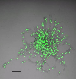
Figure 1: Depicted is an overlaid image of human U87 brain tumor cells which were stably transfected with a Green Fluorescent Protein (EGFP) Histone 2B marker for nuclei. The image is taken from a central cross-section of the MTS cultured in a three-dimensional extracellular matrix (Matrigel, Becton Dickinson, USA) environment in vitro. Note the chain-like invasive patterns. The image was taken one day post transferring the MTS from liquid medium to Matrigel (scale bar = 100 um).

Equation (11) provides the mean velocity of the tumor whenever proliferation is the only mechanism of tumor growth. However, chemotaxis drives tumor cells faster than proliferation itself, so $v_{0}$ is a small quantity. Thus, we can infer that cell proliferation is a long time process and consequently $\lambda_{M}\approx 0$ and $\lambda_{U}\approx 0$. We, therefore, assume that tumor cell proliferation is much slower than the chemotactically induced tumor cell growth (see Sec. III.2).

Equation (10) is only valid to lowest order in $\varepsilon$. Corrections to the leading behaviour of $\mu_{U}$ provide also corrections to the velocity $v_{0}$. It can be shown that xin

$$v_{0}=2(\mu_{U}\lambda_{U}K)^{1/2}(1+\xi^{1/2}),$$ (12)

where $\xi$ is obtained from the expansion of $\mu_{U}(M)$ to first order in $\varepsilon$, and can be understood as a quenched noise term, i.e., a time independent random function xin . Curvature corrections to Eq. (12) give the so-called quenched Kardar-Parisi-Zhang equation barabasi . Thus, the heterogeneity of the matrigel medium will produce rough tumor interfaces. As we will see below, some tumor fluctuations (large length scales) are amplified by chemotaxis, so they act as initial seeds for invasive branches.

III.1.2 $\mu_{M}\gg\mu_{U}$

Despite the fact that the branching morphology in Fig. 1 has been obtained in the case $\mu_{M}\ll\mu_{U}$, for completeness, we include in this section the opposite limit as well.

In this limit the diffusion coefficient of $M$ is so large that any fluctuation of $M$ is rapidly damped out. In this case, we cannot clearly separate the regions where $M$ takes its limiting values ($0$ and $M_{0}$), as was possible to do in the limit $\mu_{M}\ll\mu_{U}$ (see Fig. 2). In this case we have to deal with the full nonlinear equation that includes the dependence of $\mu_{U}$ on $M$. Hence, the specific form of the diffusion coefficient $\mu_{U}(M)$ is required in order to fully understand the evolution of the system. Müller and van Saarloos saarloos have studied the specific case in which (in our notation) $\mu_{U}(K-\lambda_{M}/\lambda_{U}U)\sim U^{k}$, with $k>0$. In such case, the gradient of the tumor field density $U$ at the boundary of the tumor is discontinuous. This could be checked experimentally in order to determine the qualitative form of the diffusion coefficient $\mu_{U}(M)$.

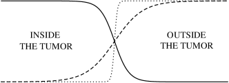
Figure 2: $M$ density field for the two limiting cases: $\mu_{M}\ll\mu_{U}$ (dotted line) and $\mu_{M}\gg\mu_{U}$ (dashed line). The solid line represents the density field of tumor cells $U$.

III.2 Growth due to heterotype chemoattraction

In this paper we are interested in the case where the nutrient medium $M$ diffuses slowly, and so the homogenization given by Eq. (10) can be assumed for all diffusion coefficients and chemotactic sensitivities. We, therefore, drop any dependence of these quantities on $M$. In what follows we restrict ourselves to a two-dimensional study, with no loss of generality (the three-dimensional analysis can be carried out as well).

As we have shown, cell proliferation cannot by itself provide invasive behaviour. The next mechanism that we must include in order to understand cell invasion is heterotype chemoattraction, where the attractant molecules are provided externally to the tumor. They diffuse rapidly until they reach the tumor boundary and then two independent events take place: the heterotype chemoattractant is degraded by the tumor cells and the tumor cells are (chemotactically) drifted to higher heterotype chemoattractant concentration gradients.

The consumption rate of the heterotype chemoattractant, $R_{Q}(Q,U)$, cannot be arbitrarily large as it saturates for large values of $Q$. This assumption is based on the concept that each tumor cell carries a finite number of $Q$-uptaking cell receptors, which in turn determine the cell’s maximum uptake rate. Besides, it is also a growing function of the tumor cell density, $U$. We do not need to specify the precise mathematical form of $R_{Q}$ at this point, but taking into account the above assumptions, we can write, without loss of generality,

$$R_{Q}(Q,U)=U^{\gamma}f(Q),$$ (13)

with $\gamma$ a positive constant.

In summary, the evolution equations in this case are

$$\partial_{t}U=\mu_{U}\nabla^{2}U-\nabla(U\chi_{Q}(Q)\nabla Q),$$ (14)

and

$$\partial_{t}Q=\mu_{Q}\nabla^{2}Q-a_{Q}U^{\gamma}f(Q),$$ (15)

where we have assumed that tumor cell proliferation is negligible compared to chemotaxis, so we can set $\lambda_{M}=\lambda_{U}=v_{0}=0$. In this limit the dynamics of $M$ is uncoupled from that of $Q$ and $U$.

Despite the fact that Eqs. (14) and (15) are highly nonlinear, due to the functions $\chi_{Q}(Q)$ and $f(Q)$, we can obtain useful information by properly rescaling space, time and both field densities $Q$ and $U$. Thus, considering an initial tumor concentration $U_{0}$ located in a bounded region of the system and a replenished source of heterotype chemoattractant modeled by Eqs. (4), we define:

$${\bf x}^{\prime} = {\bf x}\left(\frac{a_{Q}}{\mu_{Q}}\right)^{1/2},$$ (16)

$$t^{\prime} = ta_{Q},$$ (17)

$$u = U/U_{0},$$ (18)

$$q = Q/Q_{0}.$$ (19)

Eqs. (14) and (15) can be written (we drop primes for clarity) as follows

$$\partial_{t}u = \mu_{U}/\mu_{Q}\nabla^{2}u-\nu Q_{0}/\mu_{Q}\nabla(u\bar{\chi}(q)\nabla q),$$ (20)

$$\partial_{t}q = \nabla^{2}q-u^{\gamma}U_{0}^{\gamma}f(Q_{0}q)/Q_{0},$$ (21)

where $\bar{\chi}(q)$ is a dimensionless version of $\chi_{Q}(Q)$ and $\nu$ is defined through the relation $\nu\equiv\chi_{Q}(Q)/\bar{\chi}(q)$.

Note that $\mu_{Q}$ is the fastest diffusivity in the problem, so we can define an small parameter $\epsilon=\mu_{U}/\mu_{Q}$. Moreover, we also assume that the cross diffusion coefficient $\nu Q_{0}$ is smaller than $\mu_{Q}$ cross-diffusion . With these considerations Eq. (20) becomes

$$\partial_{t}u=\epsilon\nabla^{2}u-\rho\epsilon\nabla(u\bar{\chi}(q)\nabla q),$$ (22)

with $\rho=\nu Q_{0}/\mu_{U}$. Typically, the tumor field will be constant almost everywhere except in a narrow region (boundary layer nayfeh ). This region defines an interface between the inside and the outside of the tumor.

In fact, if we take the limit $\epsilon\rightarrow 0$ (the so-called outer limit nayfeh ) in Eq. (22), we have $\partial_{t}u=0$, and

$$u=\Big{\{}\begin{array}[]{lc}1&\textrm{inside the tumor,}\\ 0&\textrm{outside the tumor.}\\ \end{array}$$ (23)

One can see that in the outer limit the mathematical analysis of the problem is much simpler as Eq. (21) reduces to the equations

$$\partial_{t}q=\Big{\{}\begin{array}[]{ll}\nabla^{2}q-U_{0}^{\gamma}f(Q_{0}q)/Q_{0}&\textrm{ inside the tumor,}\\ \nabla^{2}q&\textrm{ outside the tumor.}\end{array}$$ (24)

In the case $\epsilon\neq 0$ (the so-called inner limit nayfeh ) we need to proceed with care: in order to solve Eq. (20) for $u$ and Eq. (21) for $q$, we need the behavior of $q$ exactly at the tumor boundary layer (interface). With this in mind, we define a new local set of curvilinear coordinates: a coordinate $n$ normal to the tumor interface and a coordinate $s$ tangential to it. Elementary computations (see Ref. fife ) give us the formulas for converting derivatives with respect to ${\bf x}$ to derivatives with respect to the new coordinates $(n,s)$:

$$\nabla^{2}=\partial_{nn}+\tilde{\kappa}\partial_{n}+\Delta_{s},$$ (25)

where $\tilde{\kappa}$ is the local dimensionless curvature of the tumor interface and $\Delta_{s}$ is the surface Laplacian fife . Similarly, we can write

$$\partial_{t}=\partial_{t}-\tilde{v}\partial_{n}+s_{t}\partial_{s},$$ (26)

where $\tilde{v}$ is the normal (dimensionless) velocity of the interface. We also need the following derivative

$$\nabla(u\bar{\chi}(q)\nabla q)=\partial_{n}(u\bar{\chi}(q)\partial_{n}q)+\tilde{\kappa}(u\bar{\chi}(q)\partial_{n}q)+\nabla_{s}(u\bar{\chi}(q)\nabla_{s}q).$$ (27)

Our aim now is to find solutions for $q$ and $u$ in the tumor interface. We start by rescaling the normal coordinate $n$, in terms of the fast variable $\eta=n/\epsilon$, and time in terms of $\tau=t/\epsilon$. We denote by $\tilde{u}$ and $\tilde{q}$ the inner fields, and expand them, $\bar{\chi}(\tilde{q})$ and $\tilde{v}$ in a power series of $\epsilon$ almgren :

$$\tilde{u}(\eta,s,t) = \tilde{u}_{0}+\epsilon\tilde{u}_{1}+\ldots,$$ (28)

$$\tilde{q}(\eta,s,t) = \tilde{q}_{0}+\epsilon\tilde{q}_{1}+\ldots,$$ (29)

$$\tilde{v}(\eta,s,t) = \tilde{v}_{0}+\epsilon\tilde{v}_{1}+\ldots,$$ (30)

$$\bar{\chi}(\tilde{q}) = \bar{\chi}(\tilde{q}_{0})+\bar{\chi}^{\prime}(\tilde{q}_{0})\epsilon\tilde{q}_{1}+\ldots,$$ (31)

where the prime in Eq. (31) denotes a derivative with respect to $\tilde{q}$. Using Eqs. (22),  (25),  (26) and (27), the original system of equations can be written as

$$\partial_{\tau}\tilde{u}_{0}+\epsilon\partial_{\tau}\tilde{u}_{1} = \epsilon\tilde{v}_{1}\partial_{\eta}\tilde{u}_{0}+\partial_{\eta\eta}\tilde{u}_{0}$$ (32)

$$+ \epsilon\partial_{\eta\eta}\tilde{u}_{1}-\epsilon s_{t}\partial_{s}\tilde{u}_{0}+\epsilon\tilde{\kappa}\partial_{\eta}\tilde{u}_{0}$$

$$- \rho\partial_{\eta}(\tilde{u}_{0}\bar{\chi}(\tilde{q}_{0})\partial_{\eta}\tilde{q}_{0})-\epsilon\rho\partial_{\eta}(\tilde{u}_{1}\bar{\chi}(\tilde{q}_{0})\partial_{\eta}\tilde{q}_{0})$$

$$- \epsilon\rho\partial_{\eta}(\tilde{u}_{0}\bar{\chi}(\tilde{q}_{0})\partial_{\eta}\tilde{q}_{1})-\epsilon\rho\partial_{\eta}(\tilde{u}_{0}\bar{\chi}^{\prime}(\tilde{q}_{0})\tilde{q}_{1}\partial_{\eta}\tilde{q}_{0})$$

$$- \epsilon\rho\tilde{\kappa}\tilde{u}_{0}\bar{\chi}(\tilde{q}_{0})\partial_{\eta}\tilde{q}_{0}+O(\epsilon^{2}),$$

$$\epsilon\partial_{\tau}\tilde{q}_{0} = \partial_{\eta\eta}\tilde{q}_{0}+\epsilon\partial_{\eta\eta}\tilde{q}_{1}+\epsilon\tilde{\kappa}\partial_{\eta}\tilde{q}_{0}+O(\epsilon^{2}).$$ (33)

III.2.1 Order $\epsilon^{0}$

We start by solving Eqs. (32) and (33) to order $\epsilon^{0}$. As we stated above, tumor cell proliferation is negligible when compared to chemotaxis, which means that $\tilde{v}_{0}=0$. Otherwise we have to include the reaction term $R_{M}$ in the dynamical equation for $U$ and then, to order $\epsilon^{0}$, Eq. (32) becomes:

$$\partial_{\tau}\tilde{u}_{0}+\epsilon\partial_{\tau}\tilde{u}_{1} = \tilde{v}_{0}\partial_{\eta}\tilde{u}_{0}+\epsilon\tilde{v}_{1}\partial_{\eta}\tilde{u}_{0}+\epsilon\tilde{v}_{0}\partial_{\eta}\tilde{u}_{1}+\partial_{\eta\eta}\tilde{u}_{0}$$ (34)

$$+ \epsilon\partial_{\eta\eta}\tilde{u}_{1}-\epsilon s_{t}\partial_{s}\tilde{u}_{0}+\epsilon\tilde{\kappa}\partial_{\eta}\tilde{u}_{0}$$

$$- \rho\partial_{\eta}(\tilde{u}_{0}\bar{\chi}(\tilde{q}_{0})\partial_{\eta}\tilde{q}_{0})-\epsilon\rho\partial_{\eta}(\tilde{u}_{1}\bar{\chi}(\tilde{q}_{0})\partial_{\eta}\tilde{q}_{0})$$

$$- \epsilon\rho\partial_{\eta}(\tilde{u}_{0}\bar{\chi}(\tilde{q}_{0})\partial_{\eta}\tilde{q}_{1})-\epsilon\rho\partial_{\eta}(\tilde{u}_{0}\bar{\chi}^{\prime}(\tilde{q}_{0})\tilde{q}_{1}\partial_{\eta}\tilde{q}_{0})$$

$$- \epsilon\rho\tilde{\kappa}\tilde{u}_{0}\bar{\chi}(\tilde{q}_{0})\partial_{\eta}\tilde{q}_{0}$$

$$+ \epsilon\frac{\lambda_{U}K}{a_{Q}}\left(1-\frac{\lambda_{M}U_{0}}{\lambda_{U}K}\tilde{u}_{0}\right)\tilde{u}_{0}+O(\epsilon^{2}).$$

Notice that in the absence of chemotaxis Eq. (34) becomes Fisher’s equation in the set of coordinates ($\eta,s$) and with time given by $\tau$.

From Eq. (33) we find

$$\partial_{\eta\eta}\tilde{q}_{0}=0.$$ (35)

We know that $\tilde{q}_{0}$ must be bounded at $\eta=\pm\infty$, corresponding to the inside and outside of the tumor in the scaled variable $\eta$. This implies $\partial_{\eta}\tilde{q}_{0}=0$ and, therefore, $\tilde{q}_{0}=\mathrm{constant}$. Substituting this into Eq. (32), we obtain

$$\partial_{\tau}\tilde{u}_{0}=\partial_{\eta\eta}\tilde{u}_{0},$$ (36)

which states the fact that, to first order, the tumor cells simply diffuse. Note that to this order $\tilde{u}_{0}$ does not depend on $s$, so that $\partial_{s}\tilde{u}_{0}=0$, due to the boundary conditions on $u$.

III.2.2 Order $\epsilon^{1}$

To next order in $\epsilon$ and from Eq. (33) we find,

$$\partial_{\eta\eta}\tilde{q}_{1}=0\Rightarrow\partial_{\eta}\tilde{q}_{1}=\textrm{constant},$$ (37)

due to the boundary conditions on $q$.

The next order equation for $\tilde{u}_{1}$ is given by

$$\partial_{\tau}\tilde{u}_{1}=\tilde{v}_{1}\partial_{\eta}\tilde{u}_{0}+\partial_{\eta\eta}\tilde{u}_{1}+\tilde{\kappa}\partial_{\eta}\tilde{u}_{0}-\rho(\partial_{\eta}\tilde{u}_{0})\bar{\chi}(\tilde{q}_{0})\partial_{\eta}\tilde{q}_{1}.$$ (38)

The Fredholm alternative (or solvability condition) for $\tilde{u}_{1}$ provides almgren

$$\tilde{v}_{1}=-\tilde{\kappa}+\rho B\partial_{\eta}\tilde{q}_{1},$$ (39)

where

$$B=\frac{\int_{-\infty}^{\infty}d\eta(\partial_{\eta}\tilde{u}_{0})^{2}\bar{\chi}(\tilde{q}_{0})}{\int_{-\infty}^{\infty}d\eta(\partial_{\eta}\tilde{u}_{0})^{2}}.$$ (40)

Matching the inner and outer expansions yields the normal velocity of the tumor in the original dimensions almgren :

$$v_{n}=-\mu_{U}\kappa+\nu B\nabla Q\cdot{\bf n},$$ (41)

where ${\bf n}$ is a unit vector normal to the tumor interface and directed away from the tumor.

Chemotactically induced tumor growth requires $\nabla Q\cdot{\bf n}$ to be a positive quantity, so that $v_{n}$ is positive. This can be achieved whenever the heterotype chemoattractant concentration grows as we move away from the tumor surface. Before performing the analysis of Eqs. (24) and (41) to check this requirement, we consider two interesting features related to Eq. (41). First of all, in the absence of chemotaxis and proliferation, for an initially circular tumor of radius $R_{0}$, Eq. (41) reduces to

$$\frac{dR}{dt}=-\frac{\mu_{U}}{R},$$ (42)

which gives the diffusive behavior $R(t)=\sqrt{R_{0}^{2}-2\mu_{U}t}$. This means that the mean velocity of the tumor due to diffusion decays as $t^{-1/2}$. At this stage, and for an initially circular tumor, one could now perform the following analysis: (i) suppose the tumour continues to grow as a two-dimensional disc and (ii) perturb the boundary and study the development of instabilities. This is out of the scope of this paper and will be addressed in future work. Secondly, for a general tumor front geometry, Eq. (41) provides a critical curvature, (reminiscent of the classical Greenspan model greenspan )

$$\kappa_{c}=\frac{\nu B}{\mu_{U}}\nabla Q\cdot{\bf n},$$ (43)

such that for $\kappa<\kappa_{c}$ the tumor interface has locally a positive velocity, for $\kappa>\kappa_{c}$ the tumor interface has locally a negative velocity and for $\kappa=\kappa_{c}$ the tumor interface has locally vanishing velocity. Note that this is precisely the reason of the dynamical instability that guarantees the development of invasive branches. Tumor invasion will take place on the tumor surface wherever the local curvature is below the critical value $\kappa_{c}$, given by Eq. (43). Our result agrees with the specific case considered in Ref. libro-sleeman .

As a final remark concerning Eq. (41), note that it resembles the equation for the velocity of a solidification front langer ; karma . In that case, the local normal velocity of the front depends on the local curvature, $\kappa$ as above, but on the value of the field (temperature) at the boundary, instead of the value of the gradient, $\nabla Q$, at the tumor interface. This is to be expected as in the tumor picture it is the heterotype chemoattractant that is driving the dynamics, and in the case of a solidification front, the dynamics of the front is linked to the temperature field langer ; karma . The branching behaviour of the tumor also resembles the fingering instability of the Hele-Shaw problem hele-shaw

We now turn to the requirement on the value of $\nabla Q\cdot{\bf n}$. In order to check that, indeed, $\nabla Q\cdot{\bf n}$ (or equivalently $\nabla q\cdot{\bf n}$) is a positive quantity at the tumor boundary, we need to solve Eq. (24) supplemented by Eq. (41), with initial condition,

$$q(x,y,t=0)=\delta(x-L_{x}),$$ (44)

and boundary conditions

$$q(x=0,y,t)=0,$$ (45)

$$q(x=L_{x},y,t)=1.$$ (46)

These equations cannot be solved in general without the precise form of the function $f(Q)$. Nevertheless, we may assume that, as tumor cells degrade the heterotype chemoattractant, the concentration of $q$ inside the tumor is small enough, and we can approximate $f(Q)$ by a linear function $f(Q_{0}q)\simeq\delta q$. We now proceed by solving Eq. (24) inside and outside the tumor (we denote the solutions, respectively, by $q^{-}$ and $q^{+}$) and matching both solutions at the boundary, for an initially flat tumor, i.e., a tumor for which the radius of curvature is much smaller than the system lateral size $L_{x}$ nota_flat . We first notice that $q^{+}$ is invariant under the transformation group $(L_{x}-x)\rightarrow\epsilon(L_{x}-x)$, $t\rightarrow\epsilon^{2}t$ and $q^{+}\rightarrow\epsilon^{0}q^{+}$. Similarly, $e^{\delta t}q^{-}$ is invariant under the group, $x\rightarrow\epsilon x$, $t\rightarrow\epsilon^{2}t$ and $q^{-}\rightarrow\epsilon^{0}q^{-}$. Thus, it can be straightforwardly seen that grindrod

$$q^{-}(x,y,t) = Ce^{-\delta t}\int_{0}^{x/\sqrt{t}}\,d\xi\;e^{-\xi^{2}/4},$$ (47)

$$q^{+}(x,y,t) = 1-A\int_{0}^{(L_{x}-x)/\sqrt{t}}\,d\xi\;e^{-\xi^{2}/4},$$ (48)

where $A$ and $C$ are positive constants that can be determined by continuity of the solutions at the tumor boundary ${\bf x}={\bf x_{0}}(s,t)$. As we are interested in the gradient of the $Q$ density field, we find

$$\partial_{x}q^{-}(x,y,t) = \frac{C}{\sqrt{t}}e^{-\delta t}e^{-x^{2}/4t},$$ (49)

$$\partial_{x}q^{+}(x,y,t) = \frac{A}{\sqrt{t}}e^{-(L_{x}-x)^{2}/4t}.$$ (50)

Note that Eq. (50) states that the gradient of $Q$ is a positive function, and so the tumor velocity is increased by chemotaxis as we had anticipated. Moreover, the larger the distance from $x$ to the tumor is, the larger the value of $\partial_{x}q^{+}$ becomes and the larger the value of the velocity front is (see Fig. 3). This is indeed, the reason why small fluctuations on the tumor surface become emerging invasive branches. We will see in Sec. IV that this chemotactically enhanced velocity is also obtained numerically.

Figure 3: Sketch of the heterotype chemoattractant effect on tumor cell invasive drift. Dashed lines represent level sets of $Q$ and arrows represent the local normal velocity of the tumor cells due to chemotaxis (the length of the arrows is proportional to the normal velocity).

III.3 Growth due to homotype chemoattraction

Finally, we consider the role of homotype chemoattractants. Representing protein growth factors, these chemoattractants are produced and internalized internal , or (for the purposes here), consumed by the tumor cells that move towards their positive gradients, in a similar fashion as in the heterotype case. Yet, there is no wide time scale separation between tumor and homotype chemoattractant dynamics. Thus, we cannot, in general, neglect tumor cell proliferation when analyzing homotype chemoattractant dynamics. This means that the equations in this case are Eqs. (1), (5) and (6) with $\chi_{Q}=0$. Performing a similar analysis to that of Sec. III.2 above we find:

$$v_{n}=2(\mu_{U}\lambda_{U}K)^{1/2}-\mu_{U}\kappa+\nu^{\prime}B^{\prime}\nabla C\cdot{\bf n}.$$ (51)

Despite the fact that Eq. (51) is equivalent to Eq. (41), the main differences between the evolution of $Q$ and $C$ are due to the behaviour of both density fields away from the tumor interface, namely, due to the production term $R_{C}^{(p)}$ (that is absent in the dynamical equation for $Q$) and the different boundary conditions (no external source for $C$).

Following the same steps as those carried out in Sec. III.2, we find that the outer limit yields the following equation

$$\partial_{t}c=\Big{\{}\begin{array}[]{ll}\nabla^{2}c+r^{(p)}(0,1)-r^{(d)}(c,1)&\textrm{ inside the tumor,}\\ \nabla^{2}c&\textrm{ outside the tumor,}\end{array}$$ (52)

with $r^{(p)}$ and $r^{(d)}$ scaled (dimensionless) versions of $R_{C}^{(p)}$ and $R_{C}^{(d)}$, respectively. Note that we have considered $m=0$ where $u=1$. The conservation relation given by Eq. (8) still holds in this case so, without loss of generality, we reduce the system of equations (1), (5) and (6) to Eq. (5) and Eq. (6), with $\chi_{Q}=0$ and $M$ given by Eq. (8).

Just as we did in Sec. III.2, we must now compute the sign of $\nabla C\cdot{\bf n}$ in order to determine whether or not homotype chemotaxis increases the velocity of the tumor boundary, and if it can generate a dynamical instability leading to a tumor branching morphology. We cannot in general find a transformation group under which Eq. (52) is invariant. This means that we cannot study homotype chemotaxis with the tools of the previous section. However, we can analyze homotype chemoattraction by means of its homogeneous and steady state solutions, based on generic assumptions regarding the reaction terms $R_{C}^{(p)}(M,U)$ and $R_{C}^{(d)}(C,U)$.

The homogeneous, steady state solutions (nullclines strogatz ) of equations (9) and (5) are given by the solutions of

$$R_{M}(K-\lambda_{M}/\lambda_{U}U,U) = 0,$$ (53)

$$R_{C}^{(p)}(K-\lambda_{M}/\lambda_{U}U,U) = R_{C}^{(d)}(C,U).$$ (54)

These nullclines yield the fixed points $U_{1}=0$ and $U_{2}=\lambda_{U}K/\lambda_{M}$, and $C_{1}$ and $C_{2}$ given implicitly by Eq. (54). We must distinguish between the inside and the outside of the tumor when analyzing tumor growth due to homotype chemotaxis. Outside the tumor $U_{1}=0$ and there is no production of $C$ (as there are no tumor cells). This implies that the corresponding fixed point value of $C$ is then $C_{1}=0$. On the other hand, inside the tumor, Eq. (54) reflects the fact that there is a balance between production and consumption of $C$. This means that the value of the density field $C$ reaches the fixed point $C_{2}$, which is a constant (equilibrium) value. This simple picture holds even far enough from the tumor boundary (diffusion tends to spread these uniform concentration phases). Therefore, let us consider a point in the $C-U$ plane where $U=U_{P}$ and $C=0$ (point P in Fig. 4a), namely, a point outside the tumor boundary, with $U$ so small that there has been no previous secretion of homotype chemoattractant $C$. The concentration $C$ eventually grows (as $U$ increases due to proliferation wherever $M\neq 0$) because the slope given by

$$\frac{dC}{dU}=\frac{R_{C}^{(p)}(K-\lambda_{M}/\lambda_{U}U,U)-R_{C}^{(d)}(C,U)}{R_{M}(K-\lambda_{M}/\lambda_{U}U,U)},$$ (55)

is positive note_null_1 . Then, the slope decreases note_null_2 until it reaches the nullcline where the slope is $0$ (point Q in Fig. 4a). Finally, the curve approaches the stable point $(U_{2},C_{2})$ with infinite slope (point R in Fig. 4a). Thus, $C$ grows from the outside of the tumor, reaches a maximum value and then decreases to a constant value $C_{2}$ inside the tumor. This can be schematically seen in Fig. 4b). In other words, the density field $C$ tends to grow as $U$ decreases namely, as we move outside of the tumor from inside. But, as we have shown, outside the tumor and far enough from it $C$ tends to $0$. This means that $C$ also tends to grow as we move inside of the tumor from the outside. Consequently, $C$ behaves as a pulse from the constant value $C_{2}$ inside the tumor to $C_{1}=0$ outside the tumor. This qualitative picture is sketched in Fig. 4, where we have shown that the nullcline given by Eq. (54) can have three different qualitative behaviours $N_{1}$, $N_{2}$ and $N_{3}$, that are plotted as well. This pulse-like structure for the density profile of $C$ agrees well with the intuitive picture provided in Sec. II.3. It also explains why tumor cells are chemotactically guided by the gradient of $C$. These facts will be numerically confirmed in Sec. IV below. We conclude as follows: the density profile of $C$ grows at the tumor boundary, which implies that the local normal velocity of the tumor surface increases due to the presence of a positive homotype chemoattractant gradient.

Figure 4: a) Qualitative behaviour of the trajectory of the density field $C$ in the phase-plane. The arrows indicate the direction of time evolution. Curves $N1$-$N3$ are the three types of nullclines that can be expected for our system. b) Same trajectory of the density field $C$ with respect to the spatial coordinate $x$. Again, arrows indicate time evolution.

IV Numerical study

In Sec. III we have presented a general analytical framework to study tumor growth (proliferation and chemotactic invasion). The previous analysis has been carried out by means of several assumptions and limits, (e.g., $\nu Q_{0}\ll\mu_{Q}$, $\lambda_{M}\approx 0,\lambda_{U}\approx 0$), that have not been fully justified. In this section we provide numerical simulations that check the validity of those assumptions and limits. We, thus, numerically solve the main differential equations of Sec. II following a similar organization to that of Sec. III. It is clear that in order to carry out a numerical study we must specify the detailed mathematical form of the reaction terms in our equations (1)- (6). These reaction terms are chosen following the spirit of the oncology concept previously reported in Refs. prolif ; physicaa .

IV.1 Growth due to cell proliferation

In this section, we check the validity of Eq. (8) as an approximation to Eq. (7). Thus, we have integrated Eqs. (1) and (6) with $\chi_{Q}=\chi_{C}=0$ and $R_{M}(U,M)=MU$ and, independently, Eq. (6) with $M=K-\lambda_{M}/\lambda_{U}U$.

IV.1.1 One-dimensional results

Initially, we place a one dimensional tumor such that $U(x,t=0)=1$ for $0<x<L/2$ and $U(x,t=0)=0$ elsewhere. This implies that at the initial time $M(x,t=0)=1-U(x,t=0)$. We have numerically solved Eqs. (1) and (6) with $\chi_{Q}=\chi_{C}=0$ and $R_{M}(U,M)=MU$ and, independently, Eq. (6) with $M=K-\lambda_{M}/\lambda_{U}U$. The lattice separation has been taken $dx=0.5$, the lattice size $L_{x}=128$, the diffusion coefficients $\mu_{U}=0.01$ and $\mu_{M}=0.0$, the reaction rates $\lambda_{M}=\lambda_{U}=0.1$, the time step $\epsilon_{t}=0.005$, the initial time $t_{0}=\epsilon_{t}$ and the final time $t_{f}=50000\epsilon_{t}$.

As can be seen in Fig. 5, after a small transient time, the approximation is accurate enough. As we mentioned in Sec. III, the shape of the tumor front changes slightly.

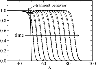
Figure 5: One dimensional tumor proliferation. Solid lines represent the $U$ density field for the model given by Eqs. (1) and (6). Dashed lines represent $U$ for the solution of Fisher’s equation, i.e., Eq. (6) with $M=K-\lambda_{M}/\lambda_{U}U$.

IV.1.2 Two-dimensional results

We now consider tumor growth due to proliferation in a two-dimensional setting with $\chi_{Q}=\chi_{C}=0$. Initially, the matrigel density $M$ is a random distribution to reflect the fact that it is an heterogeneous medium. As we are interested in a slowly varying nutrient, we choose $\varepsilon\equiv\mu_{M}/\bar{\mu}_{U}=0.01$, where $\bar{\mu}_{U}$ is the maximum attainable value of $\mu_{U}(M)$. We assume that this value of $\mu_{U}$ corresponds to the value $M=0$. The confinement due to the matrigel is unlimited, namely, for large concentrations of $M$, tumor cells can no longer diffuse. Hence, we take the following diffusion coefficient

$$\mu_{U}(M)=\frac{\bar{\mu}_{U}}{1+M/M_{\rm th}},$$ (56)

where $M_{\rm th}$ is a reference threshold concentration.

We have solved Eqs. (1) and (6) with the following initial conditions: at time $t=0$ we place a circular tumor centered at $(L_{x}/2,L_{y}/2)$ of radius $L_{x}/4$ and surrounded by a heterogeneous nutrient substrate $M$. Thus, $M(x,y,t=0)=0$ inside the initial circular tumor and $M(x,y,t=0)=1+\xi(x,y)$ elsewhere, with $\xi(x,y)$ a random Gaussian distribution with zero mean and variance $0.2$, that encodes the initial heterogeneities of the matrigel. The lattice separation has been taken $dx=dy=0.5$, the lattice size $L_{x}=L_{y}=128$, the diffusion coefficients $\bar{\mu}_{U}=0.01$ and $\mu_{M}=0.0$, the reaction rates $\lambda_{M}=\lambda_{U}=1.5$, the time step $\epsilon_{t}=0.005$, the initial time $t_{0}=\epsilon_{t}$, the final time $t_{f}=5000\epsilon_{t}$, and the intermediate times $(1000,2000,3000,4000)\epsilon_{t}$.

Figure 6 displays the time evolution of the tumor surface. Notice how the tumor conserves during its evolution its initial circular shape but develops a rough interface with the matrigel.

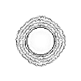
Figure 6: Numerical simulation of an initially circular tumor embedded in a matrigel medium $M$ with slow dynamics ($\mu_{M}\ll\bar{\mu}_{U}$). Different curves represent different times with the initial time $t_{0}$ corresponding to the inner perfect circle.

IV.2 Growth due to heterotype chemoattraction

The experimental branches of Fig. 1 have two characteristic lengths, namely, their width and their height with respect to the main tumor substrate. Section III.2 was devoted to determine the conditions that trigger the formation of the invasive branches. We know that the height of the branches depends in a crucial way on the mathematical form of the reaction term $R_{Q}(Q,U)$ of Eq. (2), namely, the height depends on the concentration thresholds associated with the bio-chemical reaction of $Q$ consumption by tumor cells prolif . Thus, we choose

$$a_{Q}R_{Q}(Q,U)=a_{Q}U\frac{Q}{b_{Q}+Q},$$ (57)

where $a_{Q}$ is the inverse of the time scale of consumption and $b_{Q}$ a characteristic heterotype chemoattractant concentration (threshold value). Note that, in the notation of Eq. (15) we have set $\gamma=1$.

IV.2.1 Two-dimensional results

We have integrated Eqs. (1), (6) and (2) with $R_{Q}$ given by Eq. (57) and $\chi_{C}=0$. At the initial time we place a circular tumor at $(L_{x}/2,L_{y}/2)$ with radius $L_{x}/4+\xi$, where $\xi$ is a Gaussian random number with zero mean and variance $L_{x}/20$. This initial condition mimics the effect of the slowly varying underlying substrate (matrigel) as shown in the previous section IV.1. The lattice separation has been taken $dx=dy=0.5$, the lattice size $L_{x}=L_{y}=128$, the diffusion coefficients $\mu_{U}=0.001$, $\mu_{Q}=10.0$ and $\mu_{M}=0.00001$, the reaction rates $\lambda_{M}=\lambda_{U}=0.0050$, $a_{Q}=0.75$, $b_{Q}=0.5$, the chemotactic sensitivity $\chi_{Q}=2.0$, the time step $\epsilon_{t}=0.005$, the initial time $t_{0}=\epsilon_{t}$ and the final time $t_{f}=20000\epsilon_{t}$.

Figure 7a) displays the numerically obtained tumor when the replenished source of $Q$ is placed at $x=L_{x}$ (i.e., the right hand side of the lattice). Moreover, in Fig. 7b) we show the cross-section of an invasive, chemotactically induced branch obtained in the same simulation. Clearly, we can distinguish between the main tumor spheroid and a given branch. Notice the good agreement with the experimental results and with the qualitative analysis provided in Sec. III.

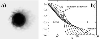
Figure 7: a) Numerical simulation of tumor branching induced by a heterotype chemotactic source located at $x=L_{x}$. The plot represents the tumor density field $U(x,y,t=20000\epsilon_{t})$. b) Cross-section of the tumor in panel a) for different times between $2000\epsilon_{t}$ and $20000\epsilon_{t}$.

IV.3 Growth due to homotype chemoattraction

The segregation and eventual degradation of the homotype chemoattractant is limited, i.e., the rates associated with both processes cannot be arbitrarily large. Thus, following Ref. physicaa we choose

$$\alpha_{C}R_{C}^{(p)}(U)=\alpha_{C}\frac{U}{\beta_{C}+U},$$ (58)

$$a_{C}R_{C}^{(d)}(C,U)=a_{C}U\frac{C}{b_{C}+C}.$$ (59)

The constants $\alpha_{C}$ and $a_{C}$ are the inverse of the characteristic time scales of production and degradation, respectively, and $\beta_{C}$ and $b_{C}$ are characteristic saturation concentrations (for production and degradation, respectively). Note the Eqs. (59) and (57) have the same mathematical form.

IV.3.1 Two-dimensional results

We have numerically integrated Eqs. (1), (6) and (5) with $\chi_{Q}=0$, and $R_{C}^{(p)}$ and $R_{C}^{(d)}$ given by Eqs. (58) and (59), respectively. The initial conditions for $U(x,y,t=0)$ are the same as those chosen in the previous section IV.2. For the matrigel and the homotype chemoattracctant, we have chosen $M(x,y,t=0)=1-U(x,y,t=0)$ and $C(x,y,t=0)=0$, respectively. The lattice separation has been taken $dx=dy=0.5$, the lattice size $L_{x}=L_{y}=128$, the diffusion coefficients $\mu_{U}=0.01$, $\mu_{C}=1.0$ and $\mu_{M}=0.0$, the reaction rates $\lambda_{M}=\lambda_{U}=0.1$, $a_{C}=1.75$, $b_{C}=0.1$, $\alpha_{C}=\beta_{C}=1.0$, the chemotactic sensitivity $\chi_{C}=1.0$, the time step $\epsilon_{t}=0.005$, the initial time $t_{0}=\epsilon_{t}$ and the final time $t_{f}=50000\epsilon_{t}$.

Fig. 8 displays the time evolution of the tumor profile in the $x$ direction for times $10000\epsilon_{t},15000\epsilon_{t},20000\epsilon_{t},25000\epsilon_{t}$ and $30000\epsilon_{t}$. The dotted line in Fig. 8 displays the $C$ profile at time $t=10000\epsilon_{t}$, magnified by a factor of $4$. In agreement with the analysis presented in section III.3, the numerical results show that (i) there is no emergence of chemotactically induced branches, as was the case for the heterotype chemoattractant and (ii) the mean speed of the tumor boundary increases due to $C$. That is, the tumor profile follows qualitatively the behaviour anticipated in Sec. III.3.

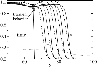
Figure 8: Cross-section of a tumor for the case of coupled dynamics between matrigel $M$, tumor cells $U$ and homotype chemoattractant $C$ for different times between $t_{0}=\epsilon_{t}$ and $t_{f}=30000\epsilon_{t}$. Solid lines: $U$ subject to homotype chemotaxis; dashed lines: $U$ subject to no homotype chemotaxis. Dotted line: $C$ (times a factor of four) for $t=10000\epsilon_{t}$.

V Discussion and Conclusions

In summary we conclude that:

1. The matrigel $M$ induces tumor cell proliferation. This growth is an overall expansion of the initial tumor that follows the principle of least resistance physicaa . Moreover, in the case of interest here, that of a slowly diffusing matrigel, the tumor boundary (or surface) becomes inhomogeneous due to the random nature of the slowly varying nutrient $M$. It is noteworthy that the roughness of the tumor surface depends also on the proliferation rate of the cells.

2. The homotype chemoattractant enhances the velocity of the tumor cells due to the increase of $C$ at the boundary of the tumor. This effect combined with cell proliferation (due to $M$) would induce the onset of invasion of tumor cells towards regions of lower matrigel density. We have been able to show that the secretion and subsequent diffusion of $C$ catalyzes the motion of the tumor cells.

3. Finally, as the heterotype chemoattractant is introduced into the system at a given distance from the tumor (in our case at the boundary), and because it diffuses, an initially circular tumor develops unstable invasive branches that move towards the source of the heterotype chemoattractant. These branches develop from initial seeds (i.e., fluctuations on the tumor boundary), which are due to the mechanical confinement from $M$, and the velocity enhancement due to $C$ and $Q$.

Our results are an improvement over sander ; physicaa . We have not limited ourselves to (i) performing a linear stability analysis from the steady state solutions as was done in sander or to (ii) numerically solving a simplified version of the reaction-diffusion equations as carried out in physicaa . On the other hand, we have analytically and numerically studied the full non-linear problem. The results of the work presented here allow us to say that proliferation is a requirement for invasion. In fact, there can be no (chemotactic) invasion without proliferation, as proliferation due to $M$ provides the initial seeds that trigger the onset of invasion. That is, the slow diffusion of $M$ is crucial to the development of those initial seeds (rough tumor interface) that become invasive branches due to heterotype chemotactically induced instability.

Admittedly, our model still does have several shortcomings as it inevitably has to simplify the complex biological scenario considered here. For instance, tumor cell apoptosis and thus, the development of a central necrotic core is currently not included necrotic . Incorporating this characteristic tumor feature would also have implications for the simulation itself. Specifically, detrimental byproducts released from the dying virtual cells would render this area “toxic”, resulting in a central space within the growing tumor, which is not being repopulated by the proliferative tumor surface. In future work, this tumor characteristic can be implemented e.g., by some dynamic, internal boundary condition within the tumor. We have also failed to model the finite receptor occupancy of the tumor cell surface. This issue is important in order to find biological support for implementing a maximum threshold of (e.g., homotype) chemoattractant uptake rate (by each tumor cell). On the other hand, the minimum threshold is given by the maximum sensitivity of the cell surface-based receptor system. Nonetheless, even in its present form the model already proves very useful for interdisciplinary cancer research as it provides the following, at least in part experimentally testable hypotheses: (i) tumor cell proliferation by itself cannot generate the invasive branching behaviour observed experimentally, yet, proliferation is a requirement for invasion (ii) heterotype chemotaxis provides an instability mechanism that leads to the onset of tumor cell invasion and (iii) homotype chemotaxis does not provide such a mechanism but enhances the mean speed of the tumor surface.

Combined with more specific experimental data, both on the molecular and on the microscopic scale, this ongoing work may therefore reveal novel and exciting insights into the role of tumor cell signaling and its impact on the emergence of multicellular patterns.

- (1) C. Betsholtz, B. Westermark, B. Ek and C. H. Heldin, Coexpression of a PDGF-like growth factor and PDGF receptors in a human osteosarcoma cell line: implications for autocrine receptor activation. Cell 39, 447-57 (1984).
- (2) J. Laterra, E. Rosen, M. Nam, S. Ranganathan, K. Fielding and P. Johnston, Scatter factor/hepatocyte growth factor expression enhances human glioblastoma tumorigenicity and growth. Biochem. Biophys. Res. Commun. 235(3), 743-7 (1997).
- (3) M. R. Chicoine, C. L. Madsen and D. L. Silbergeld, Modification of human glioma locomotion in vitro by cytokines EGF, bFGF, PDGFbb, NGF, and TNF alpha. Neurosurgery 36(6), 1165-70 (1995).
- (4) M. J. Plank, B. D. Sleeman and P. F. Jones, A mathematical model of an in vitro experiment to investigate endothelial cell migration, Jour. Theor. Medic. 4, 251-270 (2002); M. J. Plank and B. D. Sleeman, Lattice and non-lattice models of tumour angiogenesis, Bull. Math. Biol. 66, 1785-1819 (2004).
- (5) S. Koochekpour, M. Jeffers, S. Rulong, G. Taylor, E. Klineberg, E. A. Hudson, J. H. Resau and G. F. Vande Woude, Met and hepatocyte growth factor/scatter factor expression in human gliomas. Cancer Res. 57, 5391-8 (1997); A. J. Ekstrand, C. D. James, W. K. Cavenee, B. Seliger, R. F. Pettersson and V. P. Collins, Genes for epidermal growth factor receptor, transforming growth factor alpha, and epidermal growth factor and their expression in human gliomas in vivo. Cancer Res. 51(8), 2164-72 (1991).
- (6) A. Wells, Tumor invasion: role of growth factor-induced cell motility. Adv Cancer Res.78, 31-101 (2000).
- (7) L. M. Sander and T. S. Deisboeck, Phys. Rev. E 66, 051901 (2002).
- (8) T. S. Deisboeck, M. E. Berens, A. R. Kansal, S. Torquato, A. O. Stemmer-Rachamimov and E. A. Chiocca, Cell Prolif. 34, 115 (2001).
- (9) R. B. Vernon and E. H. Sage, A novel, quantitative model for study of endothelial cell migration and sprout formation within three-dimensional collage matrices. Microvasc. Res. 57, 118-133 (1999).
- (10) H. M. Byrne and M. A. J. Chaplain, Free boundary problems arising in models of tumour growth and development. Euro. Jnl. of Applied Mathematics 8, 639-658 (1998).
- (11) T. L. Jackson, S. R. Lubkin and J. D. Murray, Theoretical analysis of conjugate localization in two-step cancer chemotherapy. J. Math. Biol. 39, 353-376 (1999).
- (12) L. Preziosi, From population dynamics to modeling the competition between tumor and immune system. Math. Comp. Modelling 23, 135-152 (1996).
- (13) H. Greenspan, On the growth and stability of cell cultures and solid tumors. J. Theor. Biol. 56, 229-242 (1976).
- (14) J. P. Ward and J. R. King, Mathematical modelling of avascular-tumor growth. IMA J. Math. Appl. Med. Biol. 14, 39-69 (1997).
- (15) M. J. Holmes and B. D. Sleeman, A Mathematical Model of Tumour Angiogenesis Incorporating Cellular Traction and Viscoelastic Effects. J. Theoretical Biology 202, 45-112 (2000).
- (16) T. Alarcon, H. Byrne and P. Maini, A mathematical model of the effects of hypoxia on the cell cycle of normal and cancer cells. J. Theor. Biol. (2004).
- (17) D. S. Jones and B. D. Sleeman, Differential equations and mathematical biology (CRC Press, London) (2003) and references therein.
- (18) S. Habib, C. Molina-París and T. S. Deisboeck, Physica A 327, 501 (2003).
- (19) E. F. Keller, L. A. Segel, Model for chemotaxis. J. Theor. Biol. 30, 225-234 (1971); E. F. Keller and L. A. Segel, Traveling bands of chemotactic bacteria: a theoretical analysis. J. Theor. Biol. 30, 235-248 (1971).
- (20) J. A. Sherratt, Chemotaxis and chemokinesis in eukaryotic cells: the Keller-Segel equations as an approximation to a detailed model. Bull. Math. Biol. 56, 129-146 (1994); K. J. Painter, P. K. Maini and H. G. Othmer, Development and applications of a model for cellular response to multiple chemotactic cues. J. Math. Biol. 41, 285-314 (2000).
- (21) A. J. Ekstrand, C. D. James, W. K. Cavenee, B. Seliger, R. F. Pettersson and V. P. Collins, Genes for epidermal growth factor receptor, transforming growth factor alpha, and epidermal growth factor and their expression in human gliomas in vivo. Cancer Res. 51(8), 2164-2172 (1991).
- (22) J. Folkman and M. Hochberg, Self-regulation of growth in three dimensions. J. Exp. Med. 138, 745-753 (1973).
- (23) C. K. N. Li, The glucose distribution in 9L rat brain multicell tumor spheroids and its effect on cell necrosis. Cancer 50, 2066-2073 (1982).
- (24) J. P. Freyer, Role of necrosis in regulating the growth saturation of multicellular spheroids. Cancer Res. 48, 2432-2439 (1988).
- (25) J. P. Freyer and R. M. Sutherland, Regulation of growth saturation and development of necrosis in EMT6/Ro multicellular spheroids by the glucose and oxygen supply. Cancer Res. 46(7), 3504-3512 (1986).
- (26) H. M. Byrne and M. Chaplain, Growth of necrotic tumors in the presence and absence of inhibitors. Math. Biosci. 135 187-216 (1996).
- (27) Note that the characteristic time, , and length, , scales are related to the diffusivity through the relation . This motivates a change of variable .
- (28) J. Xin, SIAM Review 42, 161 (2000).
- (29) R. A. Fisher, Ann. Eugenics VII 355, (1936); A. Kolmogorov, I. Petrosvky and N. Piscounov, Moscow Univ. Bull. Math. A 1, 1 (1937).
- (30) Fisher’s equation has a minimal speed and a continuum of speeds , which depend on the boundary conditions. In our case we have a finite domain with no flux boundary conditions.
- (31) See A.-L. Barabási and H. E. Stanley, Fractal Concepts in Surface Growth (Cambridge University Press, Cambdridge, 1995). and references therein.
- (32) J. Müller and W. van Saarlos, Phys. Rev. E 65, 061111 (2002).
- (33) M. R. Chicoine and D. L. Silbergeld, Assessment of brain tumor cell motility in vivo and in vitro. J Neurosurg. 82(4), 615-622 (1995); R. K. Jain, Transport of molecules in the tumor interstitium: a review. Cancer Res. 47(12), 3039-51 (1987).
- (34) A. H. Nayfeh, Introduction to Perturbation Techniques (John Wiley and Sons, Mew York, 1981).
- (35) P. C. Fife, Dynamics of Internal Layers and Diffusive Interfaces, (SIAM, Philadelphia, PA, 1988).
- (36) R. F. Almgren, SIAM J. Appl. Math. 59, 2086 (1999).
- (37) J. S. Langer, Rev. Mod. Phys. 52, 1 (1980).
- (38) A. Karma and W.-J. Rappel, Phys. Rev. E 60, 3614 (1999).
- (39) P. G. Saffman and G. I. Taylor, Proc. R. Soc. London A 245, 312 (1958); D. Bensimon, L. Kadano , S. Liang, B. I. Shraiman and C. Tang, Rev. Mod. Phys. 58, 977 (1986).
- (40) We have placed the initial flat tumor at a constant value of the coordinate, that is: . This choice and the initial condition for , Eq. (44) imply that the system of equations only depends on and is independent of . We are dealing with an effectively one-dimensional system.
- (41) P. Grindrod, The Theory and Applications of Reaction-Diffusion Equations: Patterns and Waves, (Oxford University Press, New York, 1996).
- (42) F. Brightman and D. Fell, Differential feedback regulation of the MAPK cascade underlies the quantitative differences in EGF and NGF signalling in PC12 cells. FEBS Lett. 482, 169-174 (2000); B. Schoeberl, C. Eichler-Jonsson, E. D. Gilles and G. Muller, Computational modeling of the dynamics of the MAP kinase cascade activated by surface and internalized EGF receptors. Nat. Biotechnol. 20, 370-375 (2002).
- (43) S. H. Strogatz, Nonlinear Dynamics and Chaos: With Applications to Physics, Biology, Chemistry and Engineering, (Perseus Books Group,New York , 1994).
- (44) Notice that the numerator of equation (55) is positive (the production term is larger than the consumption term) and the denominator is always a positive function of both arguments.
- (45) Notice that the numerator of equation (55) is positive but decreases as increases (the consumption rate catches up with the production term ).