A Common Market Measure for Libor and Pricing Caps, Floors and Swaps in a Field Theory of Forward Interest Rates

Abstract

The main result of this paper that a martingale evolution can be chosen for Libor such that all the Libor interest rates have a common market measure; the drift is fixed such that each Libor has the martingale property. Libor is described using a field theory model, and a common measure is seen to be emerge naturally for such models. To elaborate how the martingale for the Libor belongs to the general class of numeraire for the forward interest rates, two other numeraire’s are considered, namely the money market measure that makes the evolution of the zero coupon bonds a martingale, and the forward measure for which the forward bond price is a martingale. The price of an interest rate cap is computed for all three numeraires, and is shown to be numeraire invariant. Put-call parity is discussed in some detail and shown to emerge due to some non-trivial properties of the numeraires. Some properties of swaps, and their relation to caps and floors, are briefly discussed.

1 Introduction

Libor (London Inter Bank Overnight Rates) are the interest rates for Eurodollar deposits. Libor is one of the main instruments for interest rates in the debt market, and is widely used for multifarious purposes in finance. The main focus of this paper is on the properties of Libor, and in particular finding a common measure that yields a martingale evolution [5] for all Libor. Two other numeraires for the forward interest rates are also considered, namely the money market numeraire and the forward measure for bonds.

All calculations are performed using the field theory for the forward interest rates that has been introduced in [1, 2, 3]. The main advantage of modelling the forward interest rates using field theory is that there are infinitely many random variables at each instant driving the forward rates. In particular, for the case of Libor rates, it will be shown, unlike the usual models in finance, a numeraire can be chosen so that all the Libor instruments simultaneously have a martingale evolution [4].

The price of any financial instrument in the future has to be discounted by a numeraire to obtain its current price. The freedom of choosing a numeraire results from the fact that for every numeraire there is a compensating drift such that the price of any traded instrument is independent of the numeraire. ’Numeraire invariance’ is an important tool in creating models for the pricing of financial instruments [5], and is verified by using three numeraires for pricing an interest caplet. As expected, the price of the caplet is numeraire invariant.

In Section 2 the field theory of forward rates is briefly reviewed. In Section 3 the three numeraires are discussed, and the corresponding drift velocities are evaluated. In Section 4 the price of a mid-curve interest caplet is priced for the three numeraires, in Section 5 put-call parity is derived for the three cases, in Section 6 interest swaps are discussed, and with some conclusion drawn in Section 7.

2 Field Theory Model of Forward Interest Rates

The field theory of forward rates is a general framework for modelling the interest rates that allows for a wide choice of evolution equation for the interest rates.

The Libor forward interest rates $f(t,x)$ are the interest rates, fixed at time $t$, for an instantaneous loan at future times $x>t$. Let $A(t,x)$ be a two dimensional field driving the evolution of forward rates $f(t,x)$ through time, defined by

$$\frac{\partial f(t,x)}{\partial t}=\alpha(t,x)+\sigma(t,x)A(t,x)$$ (1)

where $\alpha(t,x)$ is the drift of the forward interest rates that will be fixed by a choice of numeraire, and $\sigma(t,x)$ is the volatility that is fixed from the market [1]. One is free to choose the dynamics of how the field $A(t,x)$ evolves.

Integrating eq. 1 yields

$$f(t,x)=f(t_{0},x)+\int_{t_{0}}^{t}dt^{\prime}\alpha(t^{\prime},x)+\int_{t_{0}}^{t}dt^{\prime}\sigma(t^{\prime},x)A(t^{\prime},x)$$ (2)

where $f(t_{0},x)$ is the initial forward interest rates term structure that is specified by the market.

The price of a Libor Bond, at present time $t$, that matures at some future time $T>t$ is denoted by $B(t,T)$, and is defined in terms of the forward interest rates as follows.

$$B(t,T)=e^{-\int_{t}^{T}dxf(t,x)}$$ (3)

Following Baaquie and Bouchaud [6], the Lagrangian that describes the evolution of instantaneous Libor forward rates is defined by three parameters $\mu,\lambda,\eta$, and is given by

$${\cal L}[A]=-\frac{1}{2}\left\{A^{2}(t,z)+\frac{1}{\mu^{2}}\left(\frac{\partial A(t,z)}{\partial z}\right)^{2}+\frac{1}{\lambda^{4}}\left(\frac{\partial^{2}A(t,z)}{\partial^{2}z}\right)^{2}\right\}$$ (4)

where market (psychological) future time is defined by $z=(x-t)^{\eta}$.

The Lagrangian in eq. 4 contains a squared Laplacian term that describes the stiffness of the forward rate curve. Baaquie and Bouchaud [6] have determined the empirical values of the three constants $\mu,\lambda,\eta$, and have demonstrated that this formulation is able to accurately account for the phenomenology of Libor interest rate dynamics. Ultimately, all the pricing formulae for caps and floors depend on 1) the volatility function $\sigma(t,x)$, 2) parameters $\mu,\lambda,\eta$ contained in the Lagrangian, and lastly 3) on the initial term structure.

The action $S[A]$ and the partition function $Z$ of the Lagrangian is defined as

$$S[A] = \int_{t_{0}}^{\infty}dt\int_{0}^{\infty}dz{\cal L}[A]$$ (5)

$$Z = \int DAe^{S[A]}$$ (6)

where the symbol $\int DA$ stands for a path integral over all possible values of the quantum field $A(t,x)$.

All expectation values, denoted by $E[..]$, are evaluated by integrating over all possible values of the quantum field $A(t,z)$. The quantum theory of the forward interest rates is defined by the generating (partition) function [1] given by

$$Z[J] = E\big{[}e^{\int_{t_{0}}^{\infty}dt\int_{0}^{\infty}dzJ(t,z)A(t,z)}\big{]}$$ (7)

$$\equiv \frac{1}{Z}\int DA\,\,e^{S[A]+\int_{t_{0}}^{\infty}dt\int_{0}^{\infty}dzJ(t,z)A(t,z)}$$

$$= \exp\Big{(}\frac{1}{2}\int_{t_{0}}^{\infty}dt\int_{0}^{\infty}dzdz^{\prime}J(t,z)D(z,z^{\prime};t)J(t,z^{\prime})\Big{)}$$

All financial instruments of the interest rates are obtained by performing a path integral over the (fluctuating) two dimensional quantum field $A(t,z)$. The expectation value for an instrument, say $L[A]$, is defined by the functional average over all values of $A(t,z)$, weighted by the probability measure $e^{S}/Z$; the following notation will be used for denoting the expectation value

$$E\big{[}L[A]\big{]}\equiv\frac{1}{Z}\int DA~{}L[A]~{}e^{S[A]}$$ (8)

This a key equation that relates the formulation of finance based on stochastic calculus [8] to the one based on path integrals [1]; both formulations evaluate the same expectation values using different formalisms – in the path integral approach the averaging is carried out by performing an infinite dimensional functional integration.

For simplicity of notation, we only consider the case of $\eta=1$ and replace all integrations over $z$ with those over future time $x$.

3 Numeraire and Drift

The drift velocity $\alpha(t,x)$ is fixed by the choice of numeraire. The Libor market measure is first discussed, and then the forward measure and money market measure are discussed to elaborate different choices for the numeraire of forward rates, and the drift velocity for each is then evaluated.

3.1 Libor Market Measure

For the purpose of modeling Libor term structure, it is convenient to choose an evolution such that all the Libor rates have a martingale evolution. The deposit and payment dates are pre-fixed at 90-day intervals, denoted by $T_{n}$. The Libor forward interest rates, denoted by $L(t,T_{n})$, are simple interest rates, agreed upon at time $t<T_{n}$, for the payment that one would receive for a future time deposit from $T_{n}$ to $T_{n}+\ell$, with payments made in arrear at (future) time $T_{n}+\ell$.

In terms of the (compounded) forward interest rate Libor is given by

$$L(t,T_{n})=\frac{1}{\ell}\big{(}e^{\int^{T_{n}+\ell}_{T_{n}}dxf(t,x)}-1\big{)}$$ (9)

To understand the discounting that yields a martingale evolution of Libor rates $L(t_{0},T_{n})$ re-write Libor as follows

$$L(t,T_{n}) = \frac{1}{\ell}\big{(}e^{\int^{T_{n}+\ell}_{T_{n}}dxf(t,x)}-1\big{)}$$ (10)

$$= \frac{1}{\ell}\big{[}\frac{B(t,T_{n})-B(t,T_{n}+\ell)}{B(t,T_{n}+\ell)}\big{]}$$

The Libor is interpreted as being equal to $\big{(}B(t,T_{n})-B(t,T_{n}+\ell)\big{)}/l$, with the discounting factor for the Libor market measure being equal to $B(t,T_{n}+\ell)$. Hence, the martingale condition for the market measure, denoted by $E_{L}[..]$, is given by

$$\frac{B(t_{0},T_{n})-B(t_{0},T_{n}+\ell)}{B(t_{0},T_{n}+\ell)}=E_{L}\Big{[}\frac{B(t_{*},T_{n})-B(t_{*},T_{n}+\ell)}{B(t_{*},T_{n}+\ell)}\Big{]}$$ (11)

In other words, the market measure is defined such that each Libor is a martingale; that is, for $t_{*}>t_{0}$

$$L(t_{0},T_{n})=E_{L}[L(t_{*},T_{n})]$$ (12)

In terms of the underlying forward interest rates, the Libor’s are given by the following

$$F_{0} \equiv \int^{T_{n}+l}_{T_{n}}dxf(t_{0},x)~{}~{};~{}~{}F_{*}\equiv\int^{T_{n}+l}_{T_{n}}dxf(t_{*},x)$$ (13)

$$\Rightarrow L(t_{0},T_{n}) = \frac{1}{\ell}\big{(}e^{F_{0}}-1\big{)}~{}~{};~{}~{}L(t_{*},T_{n})=\frac{1}{\ell}\big{(}e^{F_{*}}-1\big{)}$$ (14)

and hence from eqs. 12 and 14 the martingale condition for Libor can be written as

$$e^{F_{0}}=E_{L}[e^{F_{*}}]$$ (15)

Denote the drift for the market measure by $\alpha_{L}(t,x)$, and let $T_{n}\leq x<T_{n}+\ell$; the evolution equation for the Libor forward interest rates is given, similar to eq. 2, by

$$f(t,x)=f(t_{0},x)+\int_{t_{0}}^{t}dt^{\prime}\alpha_{L}(t^{\prime},x)+\int_{t_{0}}^{t}dt^{\prime}\sigma(t^{\prime},x)A(t^{\prime},x)$$ (16)

Hence

$$E_{L}\big{[}e^{F_{*}}\big{]}=e^{F_{0}+\int_{\cal M}\alpha_{L}(t^{\prime},x)}\frac{1}{Z}\int DAe^{\int_{\cal M}\sigma(t^{\prime},x)A(t^{\prime},x)}e^{S[A]}$$ (17)

where the integration domain ${\cal M}$ is given in Fig. 1.

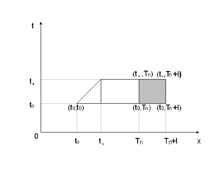
Figure 1: The domain of integration ${\cal M}$ for evaluating the drift of the Libor market numeraire.

Hence, from from eqs. 7, 15 and 17

$$e^{-\int_{\cal M}\alpha_{L}(t,x)} = \int DAe^{\int_{\cal M}\sigma(t,x)A(t,x)}e^{S[A]}$$ (18)

$$= \exp\{\frac{1}{2}\int_{t_{0}}^{t_{*}}dt\int_{T_{n}}^{T_{n}+\ell}dxdx^{\prime}\sigma(t,x)D(x,x^{\prime};t)\sigma(t,x^{\prime})\}$$

Hence the Libor drift velocity is given by

$$\alpha_{L}(t,x)=-\sigma(t,x)\int_{T_{n}}^{x}dx^{\prime}D(x,x^{\prime};t)\sigma(t,x^{\prime})~{}~{};~{}~{}T_{n}\leq x<T_{n}+\ell$$ (19)

The Libor drift velocity $\alpha_{L}(t,x)$ is negative, as is required for compensating growing payments due to the compounding of interest.

There is a discontinuity in the value of $\alpha_{L}(t,x)$ at forward time $x=T_{n}$; from its definition

$$\alpha_{L}(t,T_{n})=0$$ (20)

Approaching the value $\alpha_{L}(t,x)$ from $x>T_{n}$, the discontinuity is given by

$$\Delta\alpha_{L}(t,T_{n}) \equiv \lim_{x\rightarrow T_{n}+}\alpha_{L}(t,T_{n})-\alpha_{L}(t,T_{n})$$ (21)

$$= -\sigma(t,x)\int_{T_{n}-\ell}^{T_{n}}dx^{\prime}D(x,x^{\prime};t)\sigma(t,x^{\prime})$$

Since the time-interval for Libor $\ell=90$ days is quite small, one can approximate the drift by the following

$$\alpha_{L}(t,x)\simeq-(x-T_{n})\sigma^{2}(t,x)~{}~{};~{}~{}T_{n}\leq x<T_{n}+\ell$$ (22)

since the normalization of the volatility function can always be chosen so that $D(x,x;t)=1$ [1]. The value of discontinuity at $x=T_{n}$ is then approximately given by $-\ell\sigma^{2}(t,T_{n})$

Fig. 2 shows the behaviour of the drift velocity $\alpha_{F}(t,x)$, with the value of $\sigma(t,x)$ taken from the market [1],[11]. One can see from the graph that, in a given Libor interval, the drift velocity is approximately linear in forward time and the maximum drift goes as $\sigma^{2}(t,x)$, both of which is expected from eq. 22.

Figure 2: Negative of the drift velocity, namely $-\alpha_{L}(t,x)$, for the common Libor market measure, which is equal to the drift velocity $\alpha_{F}(t,x)$ for the forward Libor measure

3.2 Libor Forward Measure

It is often convenient to have a discounting factor that renders the futures price of Libor Bonds into a martingale. Consider the Libor forward bond given by

$$F_{L}(t_{0},T_{n+1})=e^{-\int_{T_{n}}^{T_{n+1}}dxf(t_{0},x)}=\frac{B(t_{0},T_{n+1})}{B(t_{0},T_{n})}$$ (23)

The forward numeraire is given by $B(t_{0},T_{n})$; the drift velocity is fixed so that the future price of a Libor bond is equal to its forward value; hence

$$e^{-\int_{T_{n}}^{T_{n+1}}dxf(t_{0},x)}=E_{F}\big{[}e^{-\int_{T_{n}}^{T_{n+1}}dxf(t_{*},x)}\big{]}$$ (24)

In effect, as expressed in the equation above, the forward measure makes the forward Libor bond price a martingale. To determine the corresponding drift velocity $\alpha_{F}(t,x)$, the right side of eq. 24 is explicitly evaluated. Note from eq. 2

$$E_{F}\big{[}e^{-\int_{T_{n}}^{T_{n+1}}dxf(t_{*},x)}\big{]} = e^{-\int_{T_{n}}^{T_{n+1}}dxf(t_{0},x)-\int_{\cal M}\alpha_{F}(t^{\prime},x)}\int DAe^{-\int_{\cal M}\sigma(t^{\prime},x)A(t^{\prime},x)}e^{S[A]}$$

where the integration domain ${\cal M}$ is given in Fig. 1.

Hence, from eqs. 7, 24 and 3.2

$$e^{\int_{\cal M}\alpha_{F}(t,x)} = \int DAe^{-\int_{\cal M}\sigma(t,x)A(t,x)}e^{S[A]}$$ (25)

$$= \exp\{\frac{1}{2}\int_{t_{0}}^{t_{*}}dt\int_{T_{n}}^{T_{n+1}}dxdx^{\prime}\sigma(t,x)D(x,x^{\prime};t)\sigma(t,x^{\prime})\}$$

Hence the drift velocity for the forward measure is given by

$$\alpha_{F}(t,x)=\sigma(t,x)\int_{T_{n}}^{x}dx^{\prime}D(x,x^{\prime};t)\sigma(t,x^{\prime})~{}~{};~{}~{}T_{n}\leq x<T_{n}+\ell$$ (26)

The Libor drift velocity $\alpha_{L}(t,x)$ is the negative of the drift for the forward measure, that is

$$\alpha_{F}(t,x)=-\alpha_{L}(t,x)$$

Fig. 2 shows the behaviour of the drift velocity $\alpha_{F}(t,x)$.

3.3 Money Market Measure

In Heath, Jarrow, and Morton [12], the martingale measure was defined by discounting Treasury Bonds using the money market account, with the money market numeraire $M(t,t_{*})$ defined by

$$M(t,t_{*})=e^{\int_{t}^{t_{*}}r(t^{\prime})dt^{\prime}}\,,$$ (27)

for the spot rate of interest $r(t)=f(t,t)$. The quantity $B(t,T)/M(t,t)$ is defined to be a martingale

$$\frac{B(t,T)}{M(t,t)} = E_{M}\big{[}\frac{B(t_{*},T)}{M(t,t_{*})}\big{]}$$

$$\Rightarrow B(t,T) = E_{M}\big{[}e^{-\int_{t}^{t_{*}}r(t^{\prime})dt^{\prime}}B(t_{*},T)\big{]}$$ (28)

where $E_{M}[..]$ denotes expectation values taken with respect to the money market measure. The martingale condition can be solved for it’s corresponding drift velocity, which is given by

$$\alpha_{M}(t,x)=\sigma(t,x)\int_{t}^{x}dx^{\prime}D(x,x^{\prime};t)\sigma(t,x^{\prime})$$ (29)

4 Pricing a Mid-Curve Cap

An interest rate cap is composed out of a linear sum of individual caplets. The pricing formula for an interest rate caplet is obtained for a general volatility function $\sigma(t,x)$ and propagator $D(x,x^{{}^{\prime}};t)$ that drive the underlying Libor forward rates.

A mid-curve caplet can be exercised at any fixed time $t_{*}$ that is less then the time $T_{n}$ at which the caplet matures. Denote by $Caplet(t_{0},t_{*},T_{n})$ the price – at time $t_{0}$ – of an interest rate European option contract that must be exercised at time $t_{*}>t_{0}$ for an interest rate caplet that puts an upper limit to the interest from time $T_{n}$ to $T_{n}+\ell$. Let the principal amount be equal to $\ell V$, and the caplet rate be $K$. The caplet is exercised at time $t_{*}$, with the payment made in arrears at time $T_{n}+\ell$. Note that although the payment is made at time $T_{n}+\ell$, the amount that will be paid is fixed at time $t_{*}$. The various time intervals that define the interest rate caplet are shown in Fig.3.

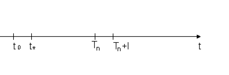
Figure 3: Time intervals in the pricing of a caplet.

The payoff function of an interest rate caplet is the value of the caplet when it matures, at $t_{0}=t_{*}$, and is given by

$$Caplet(t_{*},t_{*},T_{n}) = \ell VB(t_{*},T_{n}+\ell)\big{[}L(t_{*},T_{n})-K\big{]}_{+}$$

$$= \ell V\big{[}\frac{B(t_{*},T_{n})-B(t_{*},T_{n}+\ell)}{\ell}-KB(t_{*},T_{n}+\ell)\big{]}_{+}$$

$$= \tilde{V}B(t_{*},T_{n}+\ell)\big{(}Xe^{F_{*}}-1\big{)}_{+}$$ (31)

where recall from eq. 3.2

$$F_{*}\equiv\int_{T}^{T_{n}+\ell}dxf(t_{*},x)~{}~{}\mathrm{and}~{}~{}X=\frac{1}{1+\ell{K}}~{}~{};~{}~{}\tilde{V}=(1+\ell{K})V$$

The payoff for an interest rate floorlet is similarly given by

$$Floorlet(t_{*},t_{*},T_{n}) = \ell VB(t_{*},T_{n}+\ell)\big{[}K-L(t_{*},T_{n})\big{]}_{+}$$ (32)

$$= \tilde{V}B(t_{*},T_{n}+\ell)\big{(}1-Xe^{F_{*}}\big{)}_{+}$$

As will be shown in Section 5, the price of the caplet automatically determines the price of a floorlet due to put-call parity, and hence the price of the floorlet does not need an independent derivation.

An interest rate cap of a duration over a longer period is made from the sum over the caplets spanning the requisite time interval. Consider a mid-curve cap, to be exercised at time $t_{*}$, with strike price $K_{j}$ from time $j\ell$ to time $j(+1)\ell$, and with the interest cap starting from time $T_{m}=m\ell$ and ending at time $(n+1)\ell$; its price is given by

$$Cap(t_{0},t_{*})=\sum_{j=m}^{n}Caplet(t_{0},t_{*},T_{j};K_{j})$$ (33)

and a similar expression for an interest rate floor in terms of the floorlets for a single Libor interval.

4.1 Forward Measure Calculation for Caplet

The numeraire for the forward measure is given by the Libor Bond $B(t,T_{n})$. Hence the caplet is a martingale when discounted by $B(t,T_{n})$; the price of the caplet at time $t_{0}<t_{*}$ is consequently given by

$$\frac{Caplet(t_{0},t_{*},T_{n})}{B(t_{0},T_{n})} = E_{F}\big{[}\frac{Caplet(t_{*},t_{*},T_{n})}{B(t_{*},T_{n})}\big{]}$$

$$= \tilde{V}E_{F}\big{(}X-e^{-F_{*}}\big{)}_{+}$$

Hence, in agreement with eq. 31, the price of a caplet is given by

$$Caplet(t_{0},t_{*},T_{n})=\tilde{V}B(t_{0},T_{n})E_{F}\big{(}X-e^{-F_{*}}\big{)}_{+}$$ (34)

The payoff function for the caplet given in eq. 34 above for the interest caplet has been obtained in [1] and [13] using a different approach.

The price of the caplet is given by [1]

$$Caplet(t_{0},t_{*},T_{n})=\tilde{V}B(t_{0},T_{n})\int_{-\infty}^{+\infty}d{G}\Psi_{F}(G)(X-e^{-G})_{+}$$ (35)

From the derivation given in [1], the pricing kernel $\Psi_{F}(G)=\Psi_{F}(G,t_{0},t_{*},T_{n})$ is given by

$$\Psi_{F}(G) = \sqrt{\frac{1}{2\pi{q}^{2}}}\exp\left\{-\frac{1}{2q^{2}}\left(G-\int_{T_{n}}^{T_{n}+\ell}dx{f}(t_{0},x)-\frac{q^{2}}{2}\right)^{2}\right\}$$ (36)

$$q^{2} = q^{2}(t_{0},t_{*},T_{n})$$

$$= \int_{t_{0}}^{t_{*}}dt\int_{T_{n}}^{T_{n}+\ell}dx{d}x^{{}^{\prime}}\sigma(t,x)D(x,x^{{}^{\prime}};t)\sigma(t,x^{{}^{\prime}})$$

The price of the caplet is given by the following Black-Scholes type formula

$$Caplet(t_{0},t_{*},T_{n})=\tilde{V}B(t_{0},T)\left[X{N}(-d_{-})-{\cal F}N(-d_{+})\right]$$ (37)

where $N(d_{\pm})$ is the cumulative distribution for the normal random variable with the following definitions

$${\cal F} = e^{-\int_{T_{n}}^{T_{n}+\ell}dx{f}(t_{0},x)}=e^{-F_{0}}$$

$$d_{\pm} = \frac{1}{q}\left[\ln\left(\frac{{\cal F}}{X}\right)\pm\frac{q^{2}}{2}\right]\$$ (38)

4.2 Libor Market Measure Calculation for Caplet

The Libor market measure has as its numeraire the Libor bond $B(t_{*},T_{n}+\ell)$; the caplet is a martingale when discounted by this numeraire, and hence the price of the caplet at time $t_{0}<t_{*}$ is given by

$$\frac{Caplet(t_{0},t_{*},T_{n})}{B(t_{0},T_{n}+\ell)} = E_{L}\big{[}\frac{Caplet(t_{*},t_{*},T_{n})}{B(t_{*},T_{n}+\ell)}\big{]}$$

$$= \tilde{V}E_{L}\big{(}Xe^{F_{*}}-1\big{)}_{+}$$

$$\Rightarrow Caplet(t_{0},t_{*},T_{n}) = \tilde{V}B(t_{0},T_{n}+\ell)E_{L}\big{(}Xe^{F_{*}}-1\big{)}_{+}$$ (39)

where, similar to the derivation given in [1], the price of the caplet is given by

$$Caplet(t_{0},t_{*},T_{n}) = \tilde{V}B(t_{0},T_{n}+\ell)\int_{-\infty}^{+\infty}d{G}\Psi_{L}(G)(Xe^{G}-1)_{+}$$ (40)

For $\Psi_{L}(G)=\Psi_{L}(G,t_{0},t_{*},T_{n})$ the pricing kernel is given by

$$\Psi_{L}(G)=\sqrt{\frac{1}{2\pi{q}^{2}}}\exp\left\{-\frac{1}{2q^{2}}\left(G-\int_{T_{n}}^{T_{n}+\ell}dx{f}(t_{0},x)+\frac{q^{2}}{2}\right)^{2}\right\}$$ (41)

The price of the caplet obtained from the forward measure is equal to the one obtained using the Libor market measure since, from eqs. 35 and 36, one can prove the following remarkable result

$$B(t,T_{n})\Psi_{F}(G)(X-e^{-G})_{+}=B(t,T_{n}+\ell)\Psi_{L}(G)(Xe^{G}-1)_{+}$$ (42)

The identity above shows how the three factors required in the pricing of an interest rate caplet, namely the discount factors, the drift velocities and the payoff functions, all ‘conspire’ to yield numeraire invariance for the price of the interest rate option.

The payoff function is correctly given by the price of the caplet, since in the limit of $t_{0}\rightarrow t_{*}$, eq. 4.1 yields

$$\lim_{t_{0}\rightarrow t_{*}}q^{2} = (t_{*}-t_{0})\int_{T_{n}}^{T_{n}+\ell}dx{d}x^{{}^{\prime}}\sigma(t,x)D(x,x^{{}^{\prime}};t)\sigma(t,x^{{}^{\prime}})$$ (43)

$$= \epsilon C$$

where $C$ is a constant, and $\epsilon=t_{*}-t_{0}$. Hence, from eqs. 40 and 41

$$\lim_{t_{0}\rightarrow t_{*}}Caplet(t_{0},t_{*},T_{n}) = \tilde{V}B(t_{*},T_{n}+\ell)\int_{-\infty}^{+\infty}d{G}\delta(G-F_{*})(Xe^{G}-1)_{+}$$

$$= \tilde{V}B(t_{*},T_{n}+\ell)(Xe^{F_{*}}-1)_{+}$$

verifying the payoff function as given in eq. 31.

4.3 Money Market Calculation for Caplet

The money market numeraire is given by the spot interest rate $M(t_{0},t_{*})=exp\{\int_{t_{0}}^{t_{*}}dtr(t)\}$. Expressed in terms of the money martingale numeraire, the price of the caplet is given by

$$\frac{Caplet(t_{0},t_{*},T_{n})}{M(t_{0},t_{0})} = E_{M}\big{[}\frac{Caplet(t_{*},t_{*},T_{n})}{M(t_{0},t_{*})}\big{]}$$

$$\Rightarrow Caplet(t_{0},t_{*},T_{n}) = E_{M}\big{[}e^{-\int_{t_{0}}^{t_{*}}dtr(t)}Caplet(t_{*},t_{*},T_{n})\big{]}$$

To simplify the calculation, consider the change of numeraire from $M(t_{0},t_{*})=exp\{\int_{t_{0}}^{t_{*}}dt^{\prime}r(t^{\prime})\}$ to discounting by the Treasury Bond $B(t_{0},t_{*})$; it then follows [1] that

$$e^{-\int_{t_{0}}^{t_{*}}dtr(t)}e^{S}=B(t_{0},t_{*})e^{S_{*}}$$

where the drift for the action $S_{*}$ is given by

$$\alpha_{*}(t,x)=\sigma(t,x)\int_{t_{*}}^{x}dx^{\prime}D(x,x^{\prime};t)\sigma(t,x^{\prime})$$ (44)

In terms of the money market measure, the price of the caplet is given by

$$Caplet(t_{0},t_{*},T_{n}) = E_{M}\big{[}e^{-\int_{t_{0}}^{t_{*}}dtr(t)}Caplet(t_{*},t_{*},T_{n})\big{]}$$

$$= B(t_{0},t_{*})E_{M}^{*}\big{[}Caplet(t_{*},t_{*},T_{n})\big{]}$$

$$= \tilde{V}B(t_{0},t_{*})E_{M}^{*}\big{[}B(t_{*},T_{n}+\ell)\big{(}Xe^{F_{*}}-1\big{)}_{+}\big{]}$$

From the expression for the forward rates given in eq. 2 the price of the caplet can be written out as follows

$$Caplet(t_{0},t_{*},T_{n}) = \tilde{V}B(t_{0},t_{*})E_{M}^{*}\big{[}B(t_{*},T_{n}+\ell)\big{(}Xe^{F_{*}}-1\big{)}_{+}\big{]}$$ (46)

$$= \tilde{V}B(t_{0},T_{n}+\ell)e^{-\int_{\cal R}\alpha_{*}}~{}\frac{1}{Z}\int DAe^{-\int_{\cal R}\sigma A}e^{S_{*}}\big{(}Xe^{F_{*}}-1\big{)}_{+}$$

where the integration domain ${\cal R}$ is given in Fig. 4.

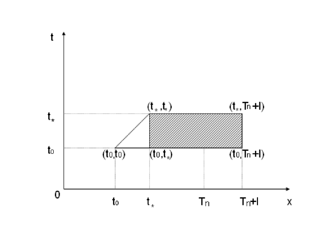
Figure 4: Domain of integration ${\cal R}$ for evaluating the price of a caplet using the money market numeraire.

The payoff can be re-expressed using the Dirac delta-function as follows

$$\big{(}Xe^{F_{*}}-1\big{)}_{+} = \int dG\delta(G-F_{*})\big{(}Xe^{G}-1\big{)}_{+}$$ (47)

$$= \int dG\int\frac{d\xi}{2\pi}e^{i\xi(G-F_{*})}\big{(}Xe^{G}-1\big{)}_{+}$$

From eq. 2, and domain of integration ${\cal M}$ given in Fig. 1, one obtains

$$F_{*} \equiv \int_{T_{n}}^{T_{n}+\ell}dxf(t_{*},x)$$

$$= \int_{T_{n}}^{T_{n}+\ell}dxf(t_{0},x)+\int_{{\cal M}}\alpha_{*}+\int_{{\cal M}}\sigma A$$

Hence, from eqs.46 and 47 the price of the caplet, for $F_{0}=\int_{T_{n}}^{T_{n}+\ell}dxf(t_{0},x)$, is given by

$$Caplet(t_{0},t_{*},T_{n}) = \tilde{V}B(t_{0},t_{*})E_{M}^{*}\big{[}B(t_{*},T_{n}+\ell)\big{(}Xe^{F_{*}}-1\big{)}_{+}\big{]}$$ (48)

$$= \tilde{V}B(t_{0},T_{n}+\ell)e^{-\int_{\cal R}\alpha_{*}}~{}\int dG\int\frac{d\xi}{2\pi}e^{i\xi(G-F_{0}-\int_{{\cal M}}\alpha_{*})}\big{(}Xe^{G}-1\big{)}_{+}\times$$

$$\frac{1}{Z}\int DAe^{-\int_{\cal R}\sigma A}e^{-i\xi\int_{{\cal M}}\sigma A}e^{S_{*}}$$

To perform path integral note that

$$\int_{\cal R}\sigma A+i\xi\int_{{\cal M}}\sigma A=\int_{t_{0}}^{t_{*}}dt\int_{t_{*}}^{T_{n}+\ell}dx\sigma(t,x)A(t,x)+i\xi\int_{t_{0}}^{t_{*}}dt\int_{T_{n}}^{T_{n}+\ell}dx\sigma(t,x)A(t,x)$$

and the Gaussian path integral using eq. 7 yields

$$\frac{1}{Z}\int DAe^{-\int_{\cal R}\sigma A-i\xi\int_{{\cal R}_{L}}\sigma A}e^{S_{*}}=e^{\Gamma}$$

where

$$\Gamma=\frac{1}{2}\int_{t_{0}}^{t_{*}}dt\int_{t_{*}}^{T_{n}+\ell}dxdx^{\prime}\sigma(t,x)D(x,x^{\prime};t)\sigma(t,x^{\prime})$$

$$~{}~{}~{}~{}~{}-\frac{\xi^{2}}{2}\int_{t_{0}}^{t_{*}}dt\int_{T_{n}}^{T_{n}+\ell}dxdx^{\prime}\sigma(t,x)D(x,x^{\prime};t)\sigma(t,x^{\prime})$$

$$~{}~{}~{}~{}~{}~{}~{}~{}~{}~{}+i\xi\int_{t_{0}}^{t_{*}}dt\int_{t_{*}}^{T_{n}+\ell}dx\int_{T_{n}}^{T_{n}+\ell}dx^{\prime}\sigma(t,x)D(x,x^{\prime};t)\sigma(t,x^{\prime})$$

The expression for $\Gamma$ above, using the definition of $q^{2},\alpha_{*}$ given in eqs. 4.1 and 44 respectively, can be shown to yield the following

$$\Gamma=\int_{\cal R}\alpha_{*}-\frac{\xi^{2}}{2}q^{2}+i\xi\big{(}\int_{{\cal M}}\alpha_{*}+\frac{1}{2}q^{2}\big{)}$$ (49)

Simplifying eq. 48 using eq. 49 yields the price of the caplet as given by

$$Caplet(t_{0},t_{*},T_{n})=\tilde{V}B(t_{0},T_{n}+\ell)\int_{-\infty}^{+\infty}d{G}\Psi_{L}(G)(Xe^{G}-1)_{+}$$ (50)

Hence we see that the money market numeraire yields the same price for the caplet as the ones obtained from the forward and Libor market measure, as expected, but with a derivation that is very different from the previous ones.

5 Put-Call Parity for Caplets and Floorlets

Put-call parity for caplets and floorlets is a model independent result, and is derived by demanding that the prices be equal of two portfolios – having identical payoffs at maturity – formed out of a caplet and the money market account on the one hand, and a floorlet and futures contract on the other hand [13]. Failure of the prices to obey the put-call parity relation would then lead to arbitrage opportunities. More precisely, put-call parity yields the following relation between the price of a caplet and a floorlet

$$Caplet(t_{0},t_{*},T_{n})+\tilde{V}B(t_{0},T_{n}+\ell)=Floorlet(t_{0},t_{*},T_{n})+\tilde{V}B(t_{0},T_{n}+\ell)Xe^{F_{0}}$$ (51)

where the other two instruments are the money market account and a futures contract.

Re-arranging eq. 51 and simplifying yields

$$Caplet(t_{0},t_{*},T_{n})-Floorlet(t_{0},t_{*},T_{n}) = \ell VB(t_{0},T_{n}+\ell)[L(t_{0},T_{n})-K]$$

$$= \mathrm{value~{}of~{}swaplet}$$

The right hand side of above equation is the price, at time $t_{0}$, of a forward or deferred swaplet, which is an interest rate swaplet that matures at time $T_{n}$; swaps are discussed in Section 6.

In this Section a derivation is given for put-call parity for (Libor) options ; the derivation is given for the three different numeraires, and illustrates how the properties are essential for the numeraires to price the caplet and floor so that they satisfy put-call parity.

The payoff for the caplet and a floorlet is generically given by

$$(a-b)_{+}=(a-b)\Theta(a-b)$$

where the Heaviside step function $\Theta(x)$ is defined by

$$\Theta(x)=\left\{\begin{array}[]{ll}1&x>0\\ \frac{1}{2}&x=0\\ 0&x<0\end{array}\right.$$ (56)

The derivation of put-call parity hinges on the following identity

$$\Theta(x)+\Theta(-x)=1$$ (57)

since it yields, for the difference of the payoff functions of the put and call options, the following

$$(a-b)_{+}-(b-a)_{+} = (a-b)\Theta(a-b)-(b-a)\Theta(b-a)$$ (58)

$$= a-b$$

5.1 Put-Call Parity for Forward Measure

The price of a caplet and floorlet at time $t_{0}$ is given by discounting the payoff functions with the discounting factor of $B(t_{0},T_{n})$. From eq. 35

$$Caplet(t_{0},t_{*},T_{n}) = B(t_{0},T_{n})E_{F}\big{[}\frac{Caplet(t_{*},t_{*},T_{n})}{B(t_{*},T_{n})}\big{]}$$

$$= \tilde{V}B(t_{0},T_{n})E_{F}\big{(}X-e^{-F_{*}}\big{)}_{+}$$

and the floorlet is given by

$$Floorlet(t_{0},t_{*},T_{n})=\tilde{V}B(t_{0},T_{n})E_{F}\big{(}e^{-F_{*}}-X\big{)}_{+}$$ (59)

Consider the expression

$$Caplet(t_{0},t_{*},T_{n})-Floorlet(t_{0},t_{*},T_{n})$$

$$= \tilde{V}B(t_{0},T_{n})\Big{[}E_{F}\big{(}X-e^{-F_{*}}\big{)}_{+}-E_{F}\big{(}e^{-F_{*}}-X\big{)}_{+}\Big{]}$$

$$= \tilde{V}B(t_{0},T_{n})E_{F}\Big{(}X-e^{-F_{*}}\Big{)}$$ (61)

where eq. 58 has been used to obtain eq. 61.

For the forward measure, from eq. 24

$$E_{F}\big{[}e^{-F_{*}}\big{]}=e^{-F_{0}}$$ (62)

Hence, since for constant $X$ we have $E_{F}(X)=XE_{F}(1)=X$, from above equation and eq. 61, the price of a caplet and floorlet obeys the put-call relation

$$Caplet(t_{0},t_{*},T_{n})-Floorlet(t_{0},t_{*},T_{n}) = \tilde{V}B(t_{0},T_{n})E_{F}\Big{(}X-e^{-F_{*}}\Big{)}$$ (63)

$$= \tilde{V}B(t_{0},T_{n})(X-e^{-F_{0}})$$

$$= \ell VB(t_{0},T_{n}+\ell)(L(t_{0},T_{n})-K)$$

and yields eq. 51 as expected.

5.2 Put-Call for Libor Market Measure

The price of a caplet for the Libor market measure is given from eq. 39 by

$$Caplet(t_{0},t_{*},T_{n})=\tilde{V}B(t_{0},T_{n}+\ell)E_{L}\big{(}Xe^{F_{*}}-1\big{)}_{+}$$ (64)

and the floorlet is given by

$$Floorlet(t_{0},t_{*},T_{n})=\tilde{V}B(t_{0},T_{n}+\ell)E_{L}\big{(}1-Xe^{F_{*}}\big{)}_{+}$$ (65)

Hence, similar to the derivation given in eq.61, we have

$$Caplet(t_{0},t_{*},T_{n})-Floorlet(t_{0},t_{*},T_{n})=\tilde{V}B(t_{0},T_{n}+\ell)E_{L}\big{(}Xe^{F_{*}}-1\big{)}$$ (66)

For the Libor market measure, from eq.15

$$E_{L}[e^{F_{*}}]=e^{F_{0}}$$

and hence equation above, together with eq. 66, yields the expected eq. 51 put-call parity relation

$$Caplet(t_{0},t_{*},T_{n})-Floorlet(t_{0},t_{*},T_{n}) = \tilde{V}B(t_{0},T_{n}+\ell)(Xe^{F_{0}}-1)$$

$$= \ell VB(t_{0},T_{n}+\ell)(L(t_{0},T_{n})-K)$$

5.3 Put-Call for Money Market Measure

The money market measure has some interesting intermediate steps in the derivation of put-call parity. Recall the caplet for the money market measure is given from eq. 48 as

$$Caplet(t_{0},t_{*},T_{n}) = E_{M}\big{[}e^{-\int_{t_{0}}^{t_{*}}dtr(t)}Caplet(t_{*},t_{*},T_{n})\big{]}$$

Using the definition of the payoff function for a caplet given in eq. 31 yields

$$Caplet(t_{0},t_{*},T_{n})=\tilde{V}E_{M}\Big{(}e^{-\int_{t_{0}}^{t_{*}}dtr(t)}\big{[}XB(t_{*},T_{n})-B(t_{*},T_{n}+\ell)\big{]}_{+}\Big{)}$$

The price of the floor is given by

$$Floorlet(t_{0},t_{*},T_{n})=\tilde{V}E_{M}\Big{(}e^{-\int_{t_{0}}^{t_{*}}dtr(t)}\big{[}B(t_{*},T_{n}+\ell)-XB(t_{*},T_{n})\big{]}_{+}\Big{)}$$

Consider the difference of put and call on a caplet; similar to the previous cases, using eq. 57 yields the following

$$Caplet(t_{0},t_{*},T_{n})-Floorlet(t_{0},t_{*},T_{n})=\tilde{V}E_{M}\Big{(}e^{-\int_{t_{0}}^{t_{*}}dtr(t)}\big{[}XB(t_{*},T_{n})-B(t_{*},T_{n}+\ell)\big{]}\Big{)}$$ (67)

The martingale condition given in eq. 28 yields the expected result given in eq. 51 that

$$Caplet(t_{0},t_{*},T_{n})-Floorlet(t_{0},t_{*},T_{n}) = \tilde{V}\big{[}XB(t_{0},T_{n})-B(t_{0},T_{n}+\ell)\big{]}$$

$$= \tilde{V}B(t_{0},T_{n}+\ell)(Xe^{F_{0}}-1)$$

$$= \ell VB(t_{0},T_{n}+\ell)(L(t_{0},T_{n})-K)$$

To obtain put-call parity for the money market account, unlike the other two cases, two instruments, namely $e^{-\int_{t_{0}}^{t_{*}}dtr(t)}B(t_{*},T_{n})$ and $e^{-\int_{t_{0}}^{t_{*}}dtr(t)}B(t_{*},T_{n}+\ell)$, have to be martingales, which in fact turned out to be the case for the money market numeraire.

6 Swaps, Caps and Floors

An interest swap is contracted between two parties. Payments are made at fixed intervals, usually $90$ or $180$ days, denoted by $T_{n}$, with the contract having notional principal $\ell V$, and a pre-fixed total duration, with the last payment made at time $T_{N}+\ell$. A swap of the first kind, namely swap_I, is where one party pays at a fixed interest rate $R_{S}$ on the notional principal, and the other party pays a floating interest rate based on the prevailing Libor rate. A swap of the second kind, namely swap_II, is where the party pays at the floating Libor rate and receives payments at fixed interest rate $R_{S}$.

To quantify the value of the swap, let the contract start at time $T_{0}$, with payments made at fixed interval $T_{n}=T_{0}+n\ell$, with times $n=0,1,2,...,N$.

Consider a swap in which the payments at the fixed rate is given by $R_{S}$; the values of the swaps are then given by [13]

$$\mathrm{swap}_{I}(T_{0},R_{S})=V\big{[}1-B(T_{0},T_{N}+\ell)-\ell R_{S}\sum_{n=0}^{N}B(T_{0},T_{n}+\ell)\big{]}$$

$$\mathrm{swap}_{II}(T_{0},R_{S})=V\big{[}\ell R_{S}\sum_{n=0}^{N}B(T_{0},T_{n}+\ell)+B(t,T_{N}+\ell)-1\big{]}$$ (68)

The par value of the swap when it is initiated, that is at time $T_{0}$, is zero; hence the par fixed rate $R_{P}$, from eq. 6, is given by [13]

$$\mathrm{swap}_{I}(T_{0},R_{P}) = 0=\mathrm{swap}_{II}(T_{0},R_{P})$$

$$\Rightarrow\ell R_{P} = \frac{1-B(T_{0},T_{N}+\ell)}{\sum_{n=0}^{N}B(T_{0},T_{n}+\ell)}$$

Recall from eqs. 5 and 33 that a cap or a floor is constructed from a linear sum of caplets and floorlets. The put-call parity for interest rate caplets and floorlets given in eq. 5 in turn yields

$$Cap(t_{0},t_{*})-Floor(t_{0},t_{*}) = \sum_{j=m}^{n}\big{[}Caplet(t_{0},t_{*},T_{j};K)-Floorlet(t_{0},t_{*},T_{j};K)\big{]}$$ (69)

$$= \ell V\sum_{n=0}^{N}B(t_{0},T_{n}+\ell)\big{[}L(t_{0},T_{n})-K\big{]}$$

The price of a swap at time $t_{0}<T_{0}$ is similar to the forward price of a Treasury Bond, and is called a forward swap or a deferred swap. Put-call parity for caps and floors gives the value of a forward swap, and hence

$$\mathrm{swap}_{I}(t_{0},R_{S})=\ell V\sum_{n=0}^{N}B(t_{0},T_{n}+\ell)\big{[}L(t,T_{n})-R_{S}\big{]}$$ (70)

$$\mathrm{swap}_{II}(t_{0},R_{S})=\ell V\sum_{n=0}^{N}B(t_{0},T_{n}+\ell)\big{[}R_{S}-L(t_{0},T_{n})\big{]}$$ (71)

The value of the swaps, from eqs. 70 and 71, can be seen to have the following intuitive interpretation: At time $T_{n}$ the value of swap_I is the difference between the floating payment received at the rate of $L(t,T_{n})$, and the fixed payments paid out at the rate of $R_{S}$. All payments are made at time $T_{n}+\ell$, and hence for obtaining its value at time $t_{0}$ need to be discounted by the bond $B(t_{0},T_{n}+\ell)$.

The definition of $L(t_{0},T_{n})$ given in eq. 10 yields the following

$$\ell V\sum_{n=0}^{N}B(t_{0},T_{n}+\ell)L(t_{0},T_{n}) = V\sum_{n=0}^{N}\big{[}B(t_{0},T_{n})-B(t_{0},T_{n}+\ell)\big{]}$$ (72)

$$= V\big{[}B(t_{0},T_{0})-B(t_{0},T_{N}+\ell)\big{]}$$

$$\Rightarrow V\big{[}1-B(T_{0},T_{N}+\ell)\big{]}~{}~{}\mathrm{for}~{}t_{0}=T_{0}$$

Hence, from eq. 70

$$\mathrm{swap}_{I}(t_{0},R_{S})=\ell V\big{[}B(t_{0},T_{0})-B(t_{0},T_{N}+\ell)-\ell R_{S}\sum_{n=0}^{N}B(t_{0},T_{n}+\ell)\big{]}$$ (73)

with a similar expression for $\mathrm{swap}_{II}$. Note that the forward swap prices, for $t_{0}\to T_{0}$, converge to the expressions for swaps given in eqs. 70 and 70.

At time $t_{0}$ the par value for the fixed rate of the swap, namely $R_{P}(t_{0})$, is given by both the forward swaps being equal to zero. Hence

$$\mathrm{swap}_{I}(t_{0},R_{P}(t_{0})) = 0=\mathrm{swap}_{II}(t_{0},R_{P}(t_{0}))$$

$$\Rightarrow\ell R_{P}(t_{0}) = \frac{B(t_{0},T_{0})-B(t_{0},T_{N}+\ell)}{\sum_{n=0}^{N}B(t_{0},T_{n}+\ell)}$$

$$= \frac{1-F(t_{0},T_{0},T_{N}+\ell)}{\sum_{n=0}^{N}F(t_{0},T_{0},T_{n}+\ell)}~{}~{}~{}~{}\mathrm{where}~{}~{}~{}F(t_{0},T_{0},T_{n}+\ell)=e^{-\int_{T_{0}}^{T_{n}+\ell}dxf(t_{0},x)}$$

$$\Rightarrow\lim_{t_{0}\to T_{0}}R_{P}(t_{0}) = R_{P}$$ (74)

We have obtained the anticipated result that the par value for the forward swap is fixed by the forward bond prices $F(t_{0},T_{0},T_{n}+\ell)$, and converges to the par value of the swap when it matures at time $t_{0}=T_{0}$.

In summary, put-call parity for cap and floor, from eqs. 69 and 70 yields, for $K=R_{S}$

$$Cap(t_{*},t_{*};R_{S})-Floor(t_{0},t_{*};R_{S})=\mathrm{swap}_{I}(t_{0},R_{S})$$ (75)

as expected [13].

7 Conclusions

A common Libor market measure was derived, and it was shown that a single numeraire renders all Libor into martingales. Two other numeraires were studied for the forward interest rates, each having its own drift velocity.

All the numeraires have their own specific advantages, and it was demonstrated by actual computation that all three yield the same price for an interest rate caplet, and also satisfy put-call parity as is necessary for the prices interest caps and floors to be free from arbitrage opportunities.

The expression for the payoff function for the caplet given in eq. 4, namely

$$Caplet(t_{0},t_{*},T_{n})=\ell VB(t_{*},T_{n}+\ell)\big{[}L(t_{*},T_{n})-K\big{]}_{+}$$

is seen to be the correct one as it reproduces the payoff functions that are widely used in the literature, yields a pricing formula for the interest rate caplet that is numeraire invariant, and satisfies the requirement of put-call parity as well.

An analysis of swaps shows that put-call parity for caps and floors correctly reproduces the swap future as expected.

8 Acknowledgements

I am greatly indebted to Sanjiv Das for sharing his insights of Libor with me, and which were instrumental in clarifying this subject to me. I would like to thank Mitch Warachka for a careful reading of the manuscript, and to Cui Liang for many discussions.

References

- [1] B. E. Baaquie, Quantum finance, Cambridge University Press (2004).
- [2] B. E. Baaquie, Physical Review E 64,016121 (2001).
- [3] B. E. Baaquie, Physical Review E 65, 056122 (2002), cond-mat/0110506.
- [4] A. Brace., D. Gatarek and M. Musiela, The Market Model of Interest Rate Dynamics, Mathematical Finance 9 (1997) 127-155.
- [5] M. Musiela and M. Rutkowski, Martingale Methods in Financial Modeling, Springer - Verlag 36 (1997).
- [6] B. E. Baaquie and J. P. Bouchaud, Stiff Interest Rate Model and Psychological Future Time Wilmott Magazine (To be published) 2004
- [7] A. Matacz and J.-P. Bouchaud, International Journal of Theoretical and Applied Finance 3, 703 (2000).
- [8] D. Lamberton, B. Lapeyre, and N. Rabeau, Introduction to Stochastic Calculus Applied to Finance. Chapman & Hill (1996).
- [9] B. E. Baaquie, M. Srikant and M. Warachka, A Quantum Field Theory Term Structure Model Applied to Hedging, International Journal of Theoretical and Applied Finance 6 (2003) 443-468.
- [10] J. P. Bouchaud, N. Sagna, R. Cont, N. El-Karoui and M. Potters, Phenomenology of the Interest Rate Curve, Applied Financial Mathematics 6 (1999) 209-232.
- [11] J. P. Bouchaud and A. Matacz, An Empirical Investigation of the Forward Interest Rate Term Structure, International Journal of Theoretical and Applied Finance 3 (2000) 703-729.
- [12] D. Heath, R. Jarrow and A. Morton, Bond Pricing and the Term Structure of Interest Rates: A New Methodology for Pricing Contingent Claims, Econometrica 60 (1992) 77-105.
- [13] R. Jarrow and S. Turnbull, Derivative Securities, Second Edition, South-Western College Publishing (2000).