Nonlinear Statistical Modelling and Model Discovery for Cardiorespiratory Data

Abstract

We present a Bayesian dynamical inference method for characterizing cardiorespiratory (CR) dynamics in humans by inverse modelling from blood pressure time-series data. This new method is applicable to a broad range of stochastic dynamical models, and can be implemented without severe computational demands. A simple nonlinear dynamical model is found that describes a measured blood pressure time-series in the primary frequency band of the CR dynamics. The accuracy of the method is investigated using surrogate data with parameters close to the parameters inferred in the experiment. The connection of the inferred model to a well-known beat-to-beat model of the baroreflex is discussed.

I Introduction

Model identification is an important method used in both fundamental and applied research Berger:89 ; Kaplan:95 ; Mullen:97 ; Mukkamala:99 ; Mukkamala:01 ; Nollo:01 ; Chon:96 ; Chon:03 on the human cardiovascular system (CVS). Because of the complexity of CVS dynamics and the multiplicity of its mechanism, it is inherently difficult or impossible to isolate and study individual response mechanisms in the intact organism Jordan:95 . In such cases mathematical models of cardiovascular control that are consistent with the experimental data can provide valuable insights Seidel:95 ; Seidel:98a . Altered dynamics of the cardiovascular system is associated with a range of cardiovascular diseases and with increased mortality, and it is hoped that dynamical metrics will provide new means of evaluating autonomic activity, and eventually form the basis for diagnostic tests for many conditions (see e.g. Berntson:97 ; Malpas:02 ; Majercak:02 ).

Despite the fact that most cardiovascular controls are demonstrably nonlinear Seidel:95 ; Sato:99 ; Stefanovska:99a ; Akselrod:00 ; Leeuwen:00 ; Malpas:01 ; Chon:03 and are perturbed by stochastic inputs Stefanovska:01b ; Stanley:02 ; Chon:03 , oversimplified assumptions of model linearity Berger:89 ; Mullen:97 ; Mukkamala:99 ; Mukkamala:01 ; Nollo:01 ; Andrew:01 ; Chon:04 and/or determinism Seidel:95 ; Akselrod:00 are often made in order to make some progress in cardiovascular system identification. Such choices are often influenced more by the availability of certain statistical tools and methodologies than by biophysical or medical considerations. It is very desirable to develop reliable methods of system identification that do not have such limitations, and are capable of treating more realistic models. Such models could be used to relate difficult-to-access parameters to non-invasively-measured data Seidel:98a .

While a number of numerical schemes have been proposed recently to deal with different aspects of the inverse problem using linear approximations Berger:89 ; Taylor:01 ; Mukkamala:01 ; Chon:01a , or semi-quantitative estimations of either the strength of some of the nonlinear terms Jamsek:03 or the directionality of coupling Rosenblum:02 ; Palus:01 , inverse cardiovascular inverse problems remain difficult because of the complexity and nonlinearity of the cardiovascular interactions, as well as the stochasticity of many dynamical inputs to the system. The problem of nonlinear cardiovascular system identification has been addressed in a number of publications Chon:96 ; Chon:01b ; Chon:03 . Nonlinearities generally require the use of more complex and involved numerical techniques McSharry:99a ; Heald:00 ; Meyer:00a ; Meyer:01 ; Rossi:02a ; Friedrich:98 ; Friedrich:03a , while the presence of dynamical noise in continuous systems can introduced systematic errors in the estimation of the model parameters Rossi:02 ; Smelyanskiy:submitted . Analogous difficulties arise in a broad range of problems in many scientific disciplines, including problems in lasers Willemsen:00a and molecular motors Visscher:99 , in epidemiology Earn:00 , and in coupled matter–radiation systems in astrophysics Christensen:02 . An obstacle to progress in these fields is the lack of general methods of dynamical inference for stochastic nonlinear systems. Accordingly the methods described in this paper should be of broad interdisciplinary interest.

In this paper we introduce a novel method for the analysis of cardiorespiratory dynamics within a nonlinear Bayesian framework for the inference of stochastic dynamical systems Smelyanskiy:submitted . This method is applied to the analysis of a univariate blood pressure time-series where a simple nonlinear dynamical model based on coupled nonlinear oscillators Saul:89a ; Stefanovska:99a ; Stefanovska:01a . is found that describes time-series data in the relevant frequency range. The accuracy of the method is investigated using surrogate data with parameters close to the parameters inferred in the experiment, and the connection of this model to a well-known beat-to-beat model of the baroreflex is discussed.

II The methodolgy

In the methodological framework presented here there are three essential steps: (i) the input data is prepared, (ii) a parameterized class of models chosen that describes the data, and (iii) the parameters of this model are inferred from the time-series data.

II.1 Data

Here we worked with a particular recording of the central venous blood pressure, a sample of which is shown in the Fig. 1(a). A feature this blood pressure (BP) time-series is the presence of the two oscillatory components at frequencies approximately $f_{r}\approx 0.2$ Hz and $f_{c}\approx 1.7$ Hz corresponding to the respiratory and cardiac oscillations. It can also be clearly seen from the spectra that the nonlinear terms including terms of nonlinear cardiorespiratory interaction (corresponding to the side peaks) are very visible in this sample. We note that the relative intensity and position of the cardiac and respiratory components vary strongly from sample to sample with average frequency of the respiration being around $0.3$ Hz and of the heart beat being around $1.1$ Hz.

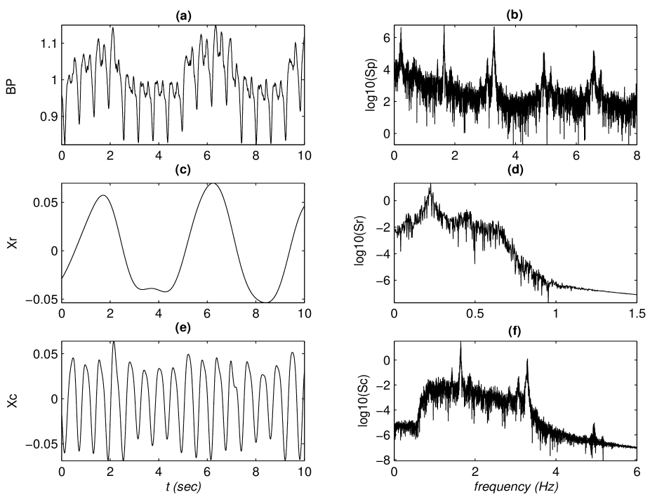
Figure 1: Data from record 24 time series of the MGH/MF Waveform Database available at www.physionet.org. (a) Original time series of the central venous blood pressure and (b) Power spectrum of original time series. (c) Respiratory component produced by filtering the blood pressure time series with a 0.06 Hz, Order 2, zero-phase, high-pass Butterworth filter and a 0.6 Hz, order 12, zero phase low-pass Butterworth filter, and (d) the power spectrum of the respiratory component. (e) Cardiac component produced by filtering the blood pressure time series with a 0.8-3.0 Hz Hz, order 8, zero-phase, band-pass Butterworth filter and (d) the power spectrum of the cardiac component. The chosen frequency range of of the components selecting according to the discussion in the text.

In preparing cardiovascular data for model identification one has to bear in mind that the CVS power spectra reflect a large variety of complex cardiovascular interactions seen as peaks and other features in a very broad frequency range Circulation:96 ; Stefanovska:97a ; Taylor:98 ; Stefanovska:01b . In order to make sense of these multi-scale phenomena parametric modelling is usually restricted to a specific part of the power spectrum. It is clear that in modelling the cardiorespiratory interaction the frequency range of modelling must include at least main harmonics of cardiac and respiratory oscillations $f_{c}$ and $f_{r}$ and their combinational frequencies. Moreover, as was pointed out already by Womersley (see e.g. Milnor:89 cf. also with Javorka:02 ) locally measured blood pressure signals resembles a steady-state oscillations and the sum of the first three harmonics contains more then 70% of the total signal variance. Therefore, it is desirable that at least three harmonics (see also discussion below) of the basic frequencies of the respiratory and cardiac oscillations are included into the frequency range of modelling.

II.2 Models

When one considers modelling the cardiovascular system, one usually envisions constructing a model based on biophysical principles that is capable of generating solutions that reproduce, to some degree, the data: the forward modelling problem (see e.g. DeBoer:87 ; Seidel:95 ; Akselrod:00 ; Stanley:02 ). One may also consider the inverse modelling problem, in which models are built that describe measured data (see e.g. Berger:89 ; Mullen:97 ; Mukkamala:99 ; Mukkamala:01 ; Chon:01b ). Both approaches have proven useful in the context of the cardiovascular research with forward approach providing valuable insight into the system and its causal relationships, and the inverse approach providing a useful means of intelligent patient monitoring of cardiovascular function.

As a third alternative one may try to bridge the two approaches by building a model that accurately reproduces the experimental observations while at the same time is based on the biophysical principles of circulation. In such a case the form of the mathematical model is taken from biophysical principles, with its component parts corresponding to a greater or lesser degree to specific biophysical mechanisms, while the values of some or all of the parameters of the mathematical model are inferred directly from from the data. In such a case it is to be hoped that information with direct biophysical significance, and not mere mathematical or statistical characterizations can be inferred from the data.

Many studies have been carried out to explore the physiological mechanisms underlying cardiorespiratory interactions Taylor:99 ; Koepchen:84 ; Melcher:76 . The most important ones are the modulation of cardiac filling pressure by respiratory movements Abel:69 , the direct respiratory modulation of parasympathetic and sympathetic neural activity in the brain stem  Gilbey:84 , and the respiratory modulation of the baroreceptor feedback control Glass:88 . A common feature that these mechanisms is that they are nonlinear, have a dynamical (or memory) component, and are subject to exogenous fluctuations  Saul:89a ; Braun:98 ; Stefanovska:99a ; Suder:98 ; Novak:93 ; Chon:96 ; Kanters:97 .

A simple beat-to-beat model describing the cardio-respiratory systems DeBoer et al. DeBoer:85 ; DeBoer:87 . The DeBoer model has further been elaborated recently in Seidel:95 ; Seidel:98a ; Stanley:02 . Insight into cardio-respiratory dynamics can also be gained through inverse modelling where the cardiac and respiratory cycles are modelled in terms of coupled nonlinear oscillators Saul:89a ; Stefanovska:97a ; Stefanovska:99a ; Stefanovska:01a ; Stefanovska:01b . In this approach spectral and synchronization features observed in the time-series data are interpreted physiologically, and related to the model parameters Stefanovska:99a . However, the identification of the model parameters could not be inferred directly from the time-series data. Instead an extensive computer simulations have been employed to establish realistic values for the model parameters Stefanovska:01b .

The simplest model that could reproduce steady-state oscillations of the blood pressure signal at two fundamental frequencies is a system of two coupled limit cycles on a plane. According to the results of the Poincar$\acute{e}$-Bendixson theory of planar dynamical systems for a system to have limit cycle in a simply connected region the divergence of the vector field must change sign in this region (see e.g. Arrowsmith:82 ). Therefore, we conclude, that the simplest system that can reproduced the discussed features of the BP signal is planar systems with limit cycles which vector field contains polynomials of the order 3. Accordingly, we model the time-series data as a system of two coupled oscillators with vector fields including nonlinearities (including nonlinearities in coupling terms) up to the 3-rd order in the form

$$\dot{x}_{r}=a_{1}x_{r}+b_{1}y_{r},\quad\dot{y}_{r}=\sum_{i=1}^{N}\alpha_{i}\phi_{i}({\bf x},{\bf y})+\sum_{j=1}^{2}\sigma_{1j}\xi_{j},$$ (1)

$$\dot{x}_{c}=a_{2}x_{c}+b_{2}y_{c},\quad\dot{y}_{c}=\sum_{i=1}^{N}\beta_{i}\phi_{i}({\bf x},{\bf y})+\sum_{j=1}^{2}\sigma_{2j}\xi_{j},$$ (2)

$$\langle\xi_{i}(t)\rangle=0,\qquad\langle\xi_{i}(t)\xi_{j}(t^{\prime})\rangle=\delta_{ij}\delta(t-t^{\prime}).$$

Here noise matrix $\sigma$ mixes zero-mean white Gaussian noises $\xi_{j}(t)$, which is related to the diffusion matrix $D=\sigma\sigma^{T}$. And base functions are chosen in the form

$$\phi=\{1,x_{r},x_{c},y_{r},y_{c},x_{r}^{2},x_{c}^{2},y_{r}^{2},y_{c}^{2},x_{r}y_{r},x_{c}y_{c},x_{r}^{3},$$

$$x_{c}^{3},x_{r}^{2}y_{r},x_{c}^{2}y_{c},x_{r}y_{r}^{2},x_{c}y_{c}^{2},y_{r}^{3},y_{c}^{3},x_{r}x_{c},x_{r}^{2}x_{c},x_{r}x_{c}^{2}\}.$$ (3)

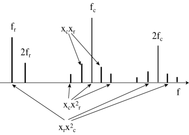
Figure 2: Summary of the main harmonics of the cardiac and respiratory components observed in the BP signal. The correspondence between the nonlinear terms of the model (1), (2) and the frequencies observed in the time-series data are shown by arrows.

The restrictions imposed on the rhs of the equations for $\dot{x}_{r}$ and $\dot{x}_{c}$ in (1) and (2) are determined mainly by the fact that we have to infer four hidden dynamical variables using univariate time-series data (see next section for further details). The parametric representation (1) and (2) covers a wide range of models with limit cycles in the plane. In particular, with a special choice of the model parameters it describes van der Pol or FitzHugh-Nagumo oscillator systems that are very popular in the context of the cardiovascular modelling. Furthermore, the choice of the parametric model in the form (1) and (2) allows one to relate them to physiological parameters characterizing autonomous nervous system (see section VI for the discussion). See Stefanovska:99a for the alternative choice and corresponding physiological reasoning.

II.3 Parameters

Following the logic of the inverse modelling approach, we must then identify the parameters ${\cal M}=\{{\bf a},{\bf b},{\bm{\alpha}},{\bm{\beta}},D\}$ of the model (1), (2) that reproduce the dynamical and spectral features of the BP signal shown in the Fig. 1. Terms representing nonlinear cardio-respiratory interactions are described by the last three base functions in (II.2). The correspondence of these terms to the experimentally observed combinational frequencies in the BP signal is summarized in the Fig. 2. It can be seen from the figure that the same combinational frequencies correspond to the nonlinear coupling terms in both limit cycle systems in the model therefore a nonlinear time-series analysis is a requirement for the identification of such a model.

Here we show how the task of identifying a model of the cardiovascular system based on coupled nonlinear oscillators can be performed systematically within a Bayesian statistical framework. In this approach parameters of the model can be inferred directly from the time-series data. We also discuss briefly how the links between the coupled oscillator model and beat-to-beat models can in principle be established.

III Bayesian inference of stochastic nonlinear dynamical models

Details of our new Bayesian technique can be found elsewhere Smelyanskiy:submitted . Here we give a brief description of the main steps of the algorithm.

Stochastic nonlinear dynamical models of the type (1), (2) can be expressed as a multi-dimensional nonlinear Langevin equation

$$\dot{\bf x}(t)={\bf f}({\bf x})+{\bf\varepsilon}(t)={\bf f}({\bf x})+{\bf\sigma}{\bf\xi}(t),$$ (4)

where ${\bf\varepsilon}(t)$ is an additive stationary white, Gaussian vector noise process characterized by

$$\langle{\bf\xi}(t)\rangle=0,\quad\langle{\bf\xi}(t)\,{\bf\xi}^{T}(t^{\prime})\rangle={\hat{\bf D}}\,\delta(t-t^{\prime}),$$ (5)

where ${\hat{\bf D}}$ is a diffusion matrix.

It is assumed that the trajectory $x(t)$ of this system is observed at sequential time instants $\{t_{k};k=0,1,\ldots,K\}$ and a series ${\cal S}=\{s_{k}\equiv s(t_{k})\}$ thus obtained is related to the (unknown) “true” system states ${\cal X}=\{x_{k}\equiv x(t_{k})\}$ through some conditional PDF $p_{\rm o}\left({\cal S}|{\cal X}\right)$.

An a priori expert knowledge about the model parameters is summarized in so-called prior PDF $p_{\textrm{pr}}({\cal M})$. In our case we chose prior in the form of zero-mean Gaussian distribution for model parameters and uniform distributions for the coefficients of diffusion matrix.

If experimental time-series data ${\cal S}$ are available they can be used to improve the estimation of the model parameters. The improved knowledge of the models parameters is summarized in the posterior conditional PDF $p_{\textrm{post}}({\cal M}|{\cal S})$, which is related to prior via Bayes’ theorem:

$$p_{\textrm{post}}({\cal M}|{\cal S})=\frac{{\ell}({\cal S}|{\cal M})\,p_{\textrm{pr}}({\cal M})}{\int\ell({\cal S}|{\cal M})\,p_{\textrm{pr}}({\cal M})\,{\rm d}{\cal M}}.$$ (6)

Here $\ell({\cal S}|{\cal M})$, usually termed the likelihood, is the conditional PDF that relates measurements ${\cal S}$ to the dynamical model. The determinant on the right hand side of the equation (6) is merely a normalization factor. In practice, (6) can be applied iteratively using a sequence of data blocks ${\cal S},{\cal S}^{\prime}$, etc. The posterior computed from block ${\cal S}$ serves as the prior for the next block ${\cal S}^{\prime}$, etc. For a sufficiently large number of observations, $p_{\textrm{post}}({\cal M}|{\cal S},{\cal S}^{\prime},\ldots)$ is sharply peaked at a certain most probable model $\cal M={\cal M}^{\ast}$.

The main efforts in the research on stochastic nonlinear dynamical inference are focused on constructing the likelihood function, which compensates noise induced errors, and on introducing efficient algorithms of optimization of the likelihood function and integration of the normalization factor (cf. McSharry:99a ; Meyer:00 ; Meyer:01 ; Rossi:02 ).

In our earlier work Smelyanskiy:submitted a novel technique of nonlinear dynamical inference of stochastic systems was introduced that solves both problems. To avoid extensive numerical methods of optimization of the likelihood function and integration of the normalization factor we suggested to parameterize the vector field of (4) in the form

$${\bf f}({\bf x})={\hat{\bf U}}({\bf x})\,{\bf c}\equiv{\bf f}({\bf x};{\bf c}),$$ (7)

where ${\hat{\bf U}}({\bf x})$ is an $N\times M$ matrix of suitably chosen basis functions $\{U_{nm}({\bf x});\,n=1:N,\,m=1:M\}$, and ${\bf c}$ is an $M$-dimensional coefficient vector. An important feature of (7) is that, while possibly highly nonlinear in ${\bf x}$, ${\bf f}({\bf x};{\bf c})$ is strictly linear in ${\bf c}$.

The computation of the likelihood function can be cast in the form of a path integral over the random trajectories of the system Graham:77 ; Dykman:90 . Using the uniform sampling scheme introduced above we can write the logarithm of the likelihood function in the following form for sufficiently small time step $h$ (cf. Graham:77 ; Dykman:90 ):

$$-\frac{2}{K}\log\ell({\bf y}|{\cal M})=\ln\det{\hat{\bf D}}+\frac{h}{K}\sum_{k=0}^{K-1}\left[\,{\bf v}({\bf y}_{k}){\bf c}\right.$$ (8)

$$\left.+(\dot{\bf y}_{k}-{\hat{\bf U}}_{k}\,{\bf c})^{T}\,{\hat{\bf D}}^{-1}\,(\dot{\bf y}_{k}-{\hat{\bf U}}_{k}\,{\bf c}))\right]+N\ln(2\pi h),$$

which relates the dynamical variables ${\bf x}(t)$ of the system (4) to the observations ${\bf s}(t)$. Here we introduce the following notations ${\bf\hat{U}}_{k}\equiv{\bf\hat{U}}({\bf y}_{k})$, $\dot{\bf y}_{k}\equiv h^{-1}({\bf y}_{k+1}-{\bf y}_{k})$ and vector ${\bf v}({\bf x})$ with components

$$\textrm{v}_{m}({\bf x})=\sum_{n=1}^{N}\frac{\partial U_{n\,m}({\bf x})}{\partial x_{n}},\quad m=1:M.$$

The vector elements $\{c_{m}\}$ and the matrix elements $\{D_{nn^{\prime}}\}$ together constitute a set ${\cal M}=\{{\bf c},{\hat{\bf D}}\}$ of unknown parameters to be inferred from the measurements ${\cal S}$.

Choosing the prior PDF in the form of Gaussian distribution

$$p_{\textrm{pr}}({\cal M})=\sqrt{\frac{\det({\bf\hat{\Sigma}}^{-1}_{\textrm{pr}})}{(2\pi)^{M}}}\exp\left(-\frac{1}{2}({\bf c}-{\bf c}_{\textrm{pr}})^{T}{\bf\hat{\Sigma}}^{-1}_{\textrm{pr}}({\bf c}-{\bf c}_{\textrm{pr}})\right).$$ (9)

and substituting $p_{\textrm{pr}}({\cal M})$ and the likelihood $\ell({\cal S}|{\cal M})$ into (6) yields the posterior $p_{\textrm{post}}({\cal M}|{\cal S})={\rm const}\times\exp[-L({\cal M}|{\cal S})]$, where

$$L({\cal M}|{\cal S})\equiv L_{\textsf{s}}({\bf c},{\bf\hat{D}})=\frac{1}{2}\rho_{\textsf{s}}({\bf\hat{D}})-{\bf c}^{T}{\bf w}_{\textsf{s}}({\bf\hat{D}})+\frac{1}{2}{\bf c}^{T}{\bf\hat{\Xi}}_{\textsf{s}}({\bf\hat{D}}){\bf c}.$$ (10)

Here, use was made of the definitions

$$\rho_{\textsf{s}}({\bf\hat{D}})=h\,\sum_{k=0}^{K-1}\dot{{\bf s}}_{k}^{T}\,{\bf\hat{D}}^{-1}\,\dot{{\bf s}}_{k}+K\,\ln(\det{\bf\hat{D}}),$$ (11)

$${\bf w}_{\textsf{s}}({\bf\hat{D}})={\bf\hat{\Sigma}}_{\textrm{pr}}^{-1}\,{\bf c}_{\textrm{pr}}+h\sum_{k=0}^{K-1}\left[{\bf\hat{U}}_{k}^{T}\,{\bf\hat{D}}^{-1}\,\dot{{\bf s}}_{k}-\frac{{\bf v}({\bf s}_{k})}{2}\right],$$ (12)

$${\bf\hat{\Xi}}_{\textsf{s}}({\bf\hat{D}})={\bf\hat{\Sigma}}^{-1}_{\textrm{pr}}+h\,\sum_{k=0}^{K-1}{\bf\hat{U}}_{k}^{T}\,{\bf\hat{D}}^{-1}\,{\bf\hat{U}}_{k}.$$ (13)

The mean values of ${\bf c}$ and ${\bf\hat{D}}$ in the posterior distribution give the best estimates for the model parameters for a given block of data ${\cal S}$ of length $K$ and provide a global minimum to $L_{\textsf{s}}({\bf c},{\hat{\bf D}})$. We handle this optimization problem in the following way. Assume for the moment that ${\bf c}$ is known in (10). Then the posterior distribution over ${\bf\hat{D}}$ has a mean ${\bf\hat{D}}^{\bf\prime}_{\textrm{post}}={\bf\hat{\Theta}}_{\textsf{s}}({\bf c})$ that provides a minimum to $S_{\textsf{s}}({\bf c},{\bf\hat{D}})$ with respect to ${\bf\hat{D}}={\bf\hat{D}}^{T}$. Its matrix elements are

$${\bf\hat{\Theta}}_{\textsf{s}}^{nn^{\prime}}({\bf c})\equiv\frac{1}{K}\,\sum_{k=0}^{K-1}\left[{\dot{\bf s}}_{k}-{\hat{\bf U}}({\bf s}_{k})\,{\bf c}\right]_{n}\left[{\dot{\bf s}}_{k}-{\hat{\bf U}}({\bf y}_{k})\,{\bf c}\right]^{T}_{n^{\prime}}.$$ (14)

Alternatively, assume next that ${\hat{\bf D}}$ is known, and note from (10) that in this case the posterior distribution over ${\bf c}$ is Gaussian. Its covariance is given by ${\bf\hat{\Xi}}_{\textsf{s}}({\bf\hat{D}})$ and the mean ${\bf c}^{\prime}_{\textrm{post}}$ minimizes $L_{\textsf{s}}({\bf c},{\bf\hat{D}})$ with respect to ${\bf c}$

$${\bf c}^{\prime}_{\textrm{post}}={\hat{\bf\Xi}}^{-1}_{\textsf{s}}({\bf\hat{D}}){\bf w}_{\textsf{s}}({\bf\hat{D}}).$$ (15)

We repeat this two-step optimization procedure iteratively, starting from some prior values ${\bf c}_{\textrm{pr}}$ and ${\bf\hat{\Sigma}}_{\textrm{pr}}$.

IV Estimation of parameters of cardiorespiratory interaction from univariate time-series data (real data)

In order to apply algorithm (12)-(15) for the identification of the model of nonlinear cardio-respiratory dynamics (1), (2) from the univariate BP time-series of the type shown in Fig. 1(a) we have to extract time-series data corresponding to the four dynamical variable in the model. Accordingly we divide the total spectrum into a low-frequency respiratory component $s_{r}(t)$ and high-frequency cardiac component $s_{c}(t)$ as is shown in Fig. 1(c) and (e).

A discussion of the physiological relevance of this spectral separation can be found in Stefanovska:99a ; Stefanovska:01a ). However, it is perfectly correct to consider this separation a mathematical ansatz. Physiological considerations need only come into play at the point where we attempt place a specific biophysical interpretation of the model elements. The parameters of the filters (see Fig. 1 caption) were chosento preserve the 2-nd and 3-rd harmonics of these signals. Then two $x_{r}(t)$ and $x_{c}(t)$ dynamical variables of the model (1), (2) can be identified with introduced above two-dimensional time-series of observations ${\bf s}(t)=\{s_{r}(t),s_{c}(t)\}$. The remaining two dynamical variables ${\bf y}(t)=\{y_{r}(t),y_{c}(t)\}$ can be related to the observations $\{{\bf s}(t_{k})\}$ as follows

$$b_{n}y_{n}(t_{k})=\frac{s_{n}(t_{k}+h)-s_{n}(t_{k})}{h}+a_{n}s_{n}(t_{k}),$$ (16)

where $n=r,c$. The relation (16) is a special form of embedding that allows one to infer a wider class of dynamical models of the cardiorespiratory interactions including models in the form of FitzHugh-Nagumo oscillators. It is clear now that we have introduced the restrictions on the form of the rhs of the first equations in (1), (2) to reduce the number of parameters of embedding that have to be selected to minimize the cost (10) and provide the best fit to the measured time series $\{{\bf s}(t_{k})\}$. The corresponding simplified model of the nonlinear interaction between the cardiac and respiratory limit cycles can now be written in the form corresponding to parametrization (7) as follows

$$\dot{\bf y}={\bf\hat{U}}({\bf s},{\bf y}){\bf c}+{\bm{\xi}}(t),$$ (17)

where ${\bm{\xi}}(t)$ is a two-dimensional Gaussian white noise with correlation matrix ${\bf\hat{D}}$, and the matrix ${\hat{\bf U}}$ will have the following block structure

$${\hat{\bf U}}=\left[\left[\begin{array}[]{ll}\phi_{1}&0\\ 0&\phi_{1}\\ \end{array}\right]\ldots\left[\begin{array}[]{ll}\phi_{2}&0\\ 0&\phi_{2}\\ \end{array}\right]\ldots\left[\begin{array}[]{ll}\phi_{B}&0\\ 0&\phi_{B}\\ \end{array}\right]\right].$$ (24)

Here $B=22$ diagonal blocks of size $2\times 2$ formed by the basis functions given in (II.2) and the vector of unknown parameters ${\bf c}$ has the length $M=2B$.

Finally, the model (17), (24) has to be inferred using method described in the previous section. The comparison between the time series of the inferred and actual cardiac oscillations is shown in Fig. 3.

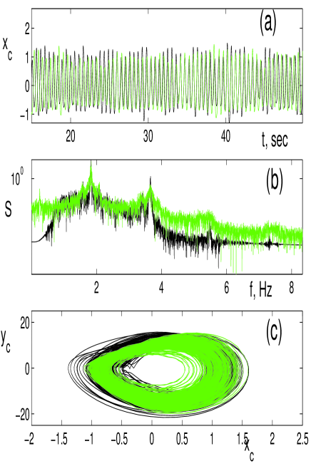
Figure 3: (a) Time series of the cardiac oscillations $x_{c}(t_{n})=s_{c}(t_{n})$ in arbitrary units (black line) obtained from central venous blood pressure. The sampling rate was 90 Hz after resampling of the original signal. Inferred time series of the cardiac oscillator (green line). (b) Power spectrum of the cardiac oscillations obtained from the real data (black line). Power spectrum of the inferred oscillations (green line). (c) Limit cycle of the cardiac oscillations $(x_{c}(n),y_{c}(n)$ obtained from real data as described in the text (black line). Limit cycle of inferred oscillations (green line).

Similar results are obtained for the respiratory oscillator as shown in the Fig. 4.

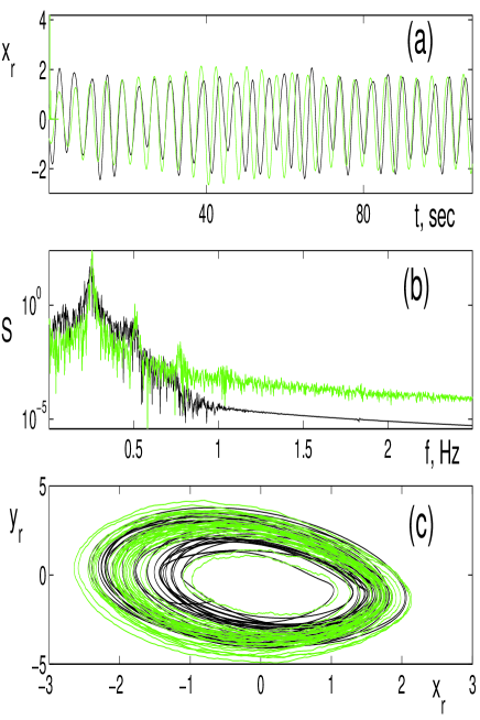
Figure 4: (a) Time series of the respiratory oscillations $x_{r}(t_{n})=s_{r}(t_{n})$ in arbitrary units (black line) obtained from central venous blood pressure. The sampling rate was 90 Hz after resampling of the original signal. Inferred time series of the respiratory oscillator (green line). (b) Power spectrum of the respiratory oscillations obtained from the real data (black line). Power spectrum of the inferred oscillations (green line). (c) Limit cycle of the respiratory oscillations $(x_{c}(n),y_{c}(n)$ obtained from real data as described in the text (black line). Limit cycle of inferred oscillations (green line).

In particular, the parameters of the nonlinear coupling and of the noise intensity of the cardiac oscillations have been estimated to have the following values $\beta_{20}=2.2,\beta_{21}=0.27$, $\beta_{22}=-8.67$, and $\langle\xi_{c}^{2}(t)\rangle=8.13$. While parameters of the coupling of respiratory oscillations to the cardiac oscillations were estimated to have the following values $\alpha_{20}=0.12,\alpha_{21}=0.048$, $\alpha_{22}=-0.066$, and $D_{11}=0.18$ . Consistent with expectations, in all experiments the parameters of the nonlinear coupling are more then one order of magnitude higher for the cardiac oscillations as compared to their values for the respiratory oscillations reflecting the fact that respiration strongly modulates cardiac oscillations, while the opposite effect of the cardiac oscillations on respiration is weak.

We have shown that it possible using these methods to simultaneously infer the coupling strengths and noise parameters nonlinear cardio-respiratory dynamics directly from a non-invasively measured time series. We view this demonstration of principle as a first step towards the practical use this technique for cardio-respiratory modelling and and in clinical applications. A number of very important physiological and mathematical issues arise in relation to the application of this new technique to specific problems. We hope to address many of these in future publications. In what follow here we specifically consider the problem of estimating of the accuracy of the method, and begin the discussion of the connection between inferred parameters and the indexes of autonomous cardiovascular controls.

V Validation of the method using surrogate time-series data

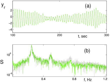
Figure 5: (a) The velocity of the respiratory component of oscillations of the original signal $y_{r}(t)$ (green line) is compared with the signal $\tilde{y}_{r}(t_{k})$ (black dashed line) obtained as a result of filtration of $s(t)$ followed by the embedding $b_{1}\tilde{y}_{r}(t_{k})=(s_{r}(t_{k}+h)-s_{r}(t_{k}))/h+a_{2}s_{r}(t_{k})$. (b) Power spectra of the original velocity of the respiratory component $y_{r}(t_{k})$ (green line) is shown in comparison with the power spectrum of the recovered signal $\tilde{y}_{r}(t_{k})$ (black dashed line).

It is desirable to check performance of the method on surrogate time-series data obtained by numerically simulating the model (1), (2)with the parameters measured with the CVS data.

To this end we consider a surrogate signal $x(t)=x_{r}(t)+x_{c}(t)$ as a time-series data input $s(t)$ for the inference. Here $x_{r}(t)$, $x_{c}(t)$ are obtained using numerical simulations of the model (1), (2) with the parameters taken from the inference of the experimental BP signal described in the previous section.

First we verify that the decomposition of the input signal $s(t)$ into low-frequency $\tilde{s}_{r}$ and high-frequency $\tilde{s}_{c}$ harmonics using two band-pass Butterworth filters and subsequent application of the embedding procedure (16) allows one to reconstruct the original signal. In the Fig. 5 we compare the velocity of the respiratory component of the original signal $y_{r}(t)$ with the the reconstructed velocity $\tilde{y}_{r}(t)$. Similar results are obtained for the reconstruction of the high-frequency component. We notice in particular that the noise introduced by embedding can be neglected since it is more then order of magnitude smaller then the dynamical noise in the signal.

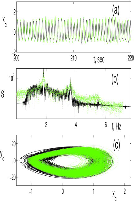
Figure 6: (a) Surrogate time series of the respiratory oscillations $x_{r}(t_{n})$ in arbitrary units (black line) obtained from model (1), (2). Inferred time series of the cardiac oscillator (green line). (b) Power spectrum of the surrogate respiratory oscillations (black line). Power spectrum of the inferred oscillations (green dashed line). (c) Limit cycle of the surrogate respiratory oscillations $(x_{c}(n),y_{c}(n)$ (black line). Limit cycle of inferred oscillations (green dashed line).

Now we can apply inference procedure described in the previous section to estimate nonlinear coupling parameters of the model from the univariate surrogate time-series data. The results of the estimation are summarized in the Table 1.

$\alpha_{20}$	$\beta_{20}$	$\alpha_{21}$	$\beta_{21}$	$\alpha_{22}$	$\beta_{22}$	$D_{11}$	$D_{22}$
0.12	2.2	0.048	0.27	-0.066	-8.67	0.18	8.13
0.18	6.32	0.011	0.49	0.053	6.03	0.017	3.44
51.2%	186.8%	75.9%	102.7%	27.9%	30.6%	90.8%	57.7%

Table 1: Absolute values of the coefficients of nonlinear cardiorespiratory interactions corresponding to the last three base functions (II.2) $\{x_{r}x_{c},x_{r}^{2}x_{c},x_{r}x_{c}^{2}\}$. Coefficients $\{\alpha_{i}\}$ correspond to the respiration coupling to cardiac rhythm. Coefficients $\{\beta_{i}\}$ correspond to the cardiac oscillation coupling to respiration. For each set of coefficients the actual values (top row) are compared with the mean inferred values obtained from 100 blocks of time-series data $x(t)=x_{r}(t)+x_{c}(t)$ with 50000 points in each block and sampling time 0.02 sec (middle row). The error of estimation is shown in the bottom line.

It can be seen from the table that the method allows one to estimate correct order of the absolute values of the nonlinear coupling parameter. For some parameter the accuracy of the estimation is much better, but in practice the correct values are not know. Therefore we conclude that the accuracy of the estimation of the absolute values of parameters of coupling of two limit cycle systems from univariate time-series data is within the order of magnitude.

$\alpha_{20}$	$\beta_{20}$	$\alpha_{21}$	$\beta_{21}$	$\alpha_{22}$	$\beta_{22}$	$D_{11}$	$D_{22}$
0.12	2.20	0.048	0.27	-0.066	-8.67	0.18	8.13
0.12	2.41	0.048	0.28	-0.070	-8.61	0.18	8.14
2.9%	9.3%	1.8%	5.6%	5.2%	0.7%	0.2%	0.2%

Table 2: Absolute values of the coefficients of nonlinear cardiorespiratory interactions corresponding to the last three base functions (II.2) $\{x_{r}x_{c},x_{r}^{2}x_{c},x_{r}x_{c}^{2}\}$. Coefficients $\{\alpha_{i}\}$ correspond to the respiration coupling to cardiac rhythm. Coefficients $\{\beta_{i}\}$ correspond to the cardiac oscillation coupling to respiration. For each set of coefficients the actual values (top row) are compared with the mean inferred values obtained from 100 blocks of time-series data $\{x_{r}(t),x_{c}(t),y_{r}(t),y_{c}(t)\}$ with 160000 points in each block and sampling time 0.01 sec (middle row). The error of estimation is shown in the bottom line.

Similar results are obtained for the estimation of other parameters of the model. Using values of the model parameters estimated from the univariate surrogate data one can reconstruct very closely the dynamical and spectral features of the original system as shown in the Fig. 6. The largest errors of estimations are obtained for the values of the noise intensity as shown in two last columns of the Table 6. This result can be easily understood taking into account that filtration of the signals has the strongest effect on the noise spectrum of the system. However, the filter-induced errors are systematic and can be corrected using test with surrogate data.

The main source of error is related to the spectral decomposition of the univariate data and it is therefore systematic. To illustrate this point we use the original surrogate time-series data $\{x_{r}(t),x_{c}(t),y_{r}(t),y_{c}(t)\}$ for two coupled oscillators to infer parameters of the model (1), (2). The results of inference of the coupling parameters are shown in the Tab. 2. It can be seen that the values of the parameters can be estimated with relative error better then 10%. In particular, the relative error of estimation of the noise intensity is now better then 4%. The accuracy of the estimation can be further improved by increasing the total time of observation of the system dynamics as explained in Smelyanskiy:submitted .

These results should be compared with semi-quantitative estimations of either relative strength of some of the nonlinear terms Jamsek:03 or the directionality of coupling Rosenblum:02 ; Palus:01 from bivariate time-series data. It becomes clear that our algorithm provides an alternative effective approach to the solution of the problem of analysis of cardiovascular coupling. In particular, the results of this section validate the application of the method to the experimental time-series cardiovascular data and demonstrate that the it is indeed possible to estimate simultaneously the strength, directionality and the noise of nonlinear cardiorespiratory coupling form the univariate blood pressure signal. The accuracy of the estimation is within the order of the magnitude. The main source of errors is the decomposition of the univariate signal into two oscillatory components and it is, therefore, systematic. Using this fact one can introduce systematic corrections to improve the results of the estimation of the parameters of the CR interaction from the experimentally measured BP signal.

VI Discussion

It is important to establish a relationship between the model parameters and physiological parameters of the cardiovascular system. A beat-to-beat model describing the relationships between blood pressures and respiration in simple, but physiologically meaningful terms is the DeBoer model DeBoer:85 ; DeBoer:87 . While the DeBoer model cannot describe the dynamics within one heartbeat it does incorporate several well-known physiological laws of the cardio-respiratory system. More recent extensions and modifications of the DeBoer model have appeared Seidel:95 ; Seidel:98a ; Stanley:02 . The problem of inverse modelling was not addressed in this earlier work. It is therefore very desirable to connect the approach presented here with such beat-to-beat models.

The DeBoer model describes the beat-to-beat evolution of the state variables shown in the Fig. 7 (a): systolic pressure ($S$), diastolic pressure ($D$), RR intervals ($I$), and arterial decay time ($T=R\times C=$ peripheral resistance $\times$ arterial compliance). Following a brief account of the DeBoer model given in Akselrod:00 and neglecting for the sake of simplicity the variation of the peripheral resistance we can write a set of corresponding difference equations in the form

$$D_{i} = S_{i-1}\exp[(-2/3)I_{i-1}/T],$$ (25)

$$S_{i} = D_{i}+\gamma I_{i-1}+C_{1}+A\sin(2\pi ft),$$ (26)

$$I_{i} = G_{v}S^{\prime}_{i-\tau_{v}}+G_{\beta}F(S^{\prime},\tau_{\beta})+C_{2},$$ (27)

Here $C_{1}$, $C_{2}$, and $C_{3}$ are constants and the sigmoidal nature of the baroreceptor sensitivity is accounted for by defining an effective Systolic pressure ($S^{\prime}$) DeBoer:87

$$S^{\prime}_{i}=S_{0}+18\arctan[(S-S_{0})/18].$$ (28)

The first equation (25) follows from the Windkessel model of the circulation, while the second equation (26) expresses contractile properties of the myocardium in accordance with Starling’s law that takes into account mechanical effect of the circulation on the BP (see DeBoer:87 and e.g. Milnor:89 ). The last equation (27) includes explicitly two mechanisms of the cardiovascular control defined by their respective gain ($G$) and delay ($\tau$): (i) fast vagal control of the heart rate $G_{v}S^{\prime}_{i-\tau_{v}}$, (ii) slower $\beta$-sympathetic control of the heart rate $G_{\beta}F(S^{\prime},\tau_{\beta})$. Here $F(S^{\prime},\tau)$ is a linear weighted sum of the form

$$F(S^{\prime},\tau)=\sum_{k=-M}^{M}a_{k}S^{\prime}_{i-\tau+k}=(S^{\prime}_{i-\tau-2}+2S^{\prime}_{i-\tau-1})$$

$$+3S^{\prime}_{i-\tau}+2S^{\prime}_{i-\tau+1}+S^{\prime}_{i-\tau+2})/9$$

Further we assume for simplicity that the pressure oscillations do not deviate far away from the working point $S_{0}$ in (28), i.e. $S^{\prime}\approx S$.

To establish the connection between DeBoer (25) - (27) model and the model (1), (2) introduced in this paper we note that the equations DeBoer model is a piece-wise approximation of the actual BP signal. In particular, it describes the BP signal as an exponential decay during 2/3 part of the $RR$ interval and linear increase during 1/3 of the $I_{n}$ as show in the Fig. 7 (b).

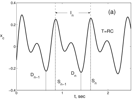
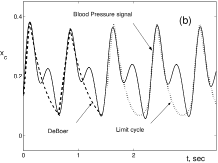
Figure 7: (a) The BP signal in the frequency range of cardiac oscillations (black line). Systolic pressure ($S_{n}$), diastolic pressure ($D_{n}$), RR intervals ($I_{n}$), and arterial decay time ($T=RC=$) are shown for the $n$-th heartbeat. (b) Comparison of the BP signal (thing black line) with the approximation adopted in the DeBoer model (dashed line) and the approximation by the FitzHugh-Nagumo model (dotted line). Vertical scale has arbitrary units.

We note also that the model of the cardiac oscillations (2) resembles a model of the FitzHugh-Nagumo (FHN) system

$$\left\{\begin{array}[]{ll}\dot{x}&=\epsilon(y-\beta x),\\ \dot{y}&=\alpha y+\gamma y^{2}+\delta y^{3}-x+C,\\ \end{array}\right.$$ (31)

where we have neglected for a moment the cardiorespiratory interaction. The approximation of the BP signal by the output of the FHN system is also shown in the Fig. 7 (b). It can be seen already from a comparison between two approximations that there is a close connections between DeBoer model and model of coupled oscillators considered in this paper. This can be further illustrated by noticing that for small $\epsilon$ the limit cycle in the FHN system consists of fast motion with practically constant values of $y$, when $x$ jumps between negative and positive values, and slow motion, when $x$ changes very little (see Fig. 8). Assuming the constant value of $x$ at the top $|a_{+}|$ and at the bottom $-|a_{-}|$ of the dashed curve that correspond to the slow motion along the limit cycle we can integrate the first equation in (31) to obtain

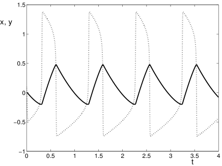
Figure 8: Time evolution of the dynamical variables $x$ (solid line) and $y$ (dashed line) of the FHN system with the following parameters: $\epsilon=0.01$, $\beta=-0.05$, $C=-0.125$, $\alpha=0.5$, $\gamma=1$, $\delta=-1$.

$$x_{0}(t)=\left\{\begin{array}[]{ll}(S_{n-1}-|a_{-}|)e^{-\beta t}+|a_{-}|,&\hbox{for $0<t<\frac{2}{3}I_{n}$;}\\ (D_{n}+|a_{+}|)e^{-\beta t}-|a_{+}|,&\hbox{for $\frac{2}{3}I_{n}<t<I_{n}$.}\\ \end{array}\right.$$

This solution closely resembles eqs. (25) and (26) of the DeBoer model

It can be seen even from this simplified discussion that the parameters of the model (1), (2) found in the present paper can be related directly to the physiological parameters of the autonomous control of circulation. Furthermore, this discussion suggests that it should be possible at least in principle to bridge inverse and forward modelling and to infer parameters of the autonomous nervous control of the cardiovascular system directly from the time-series data.

We emphasize, however, that the obtained results is only the first step in this direction. In particular, the DeBoer model itself has to be modified in various ways, including more realistic functional form of the feedback terms and specifically taking into account the fact that the baroreflex control is a closed loop Sato:99 ; Malpas:01 . In fact it was shown Heldt:02 that a multi-compartment closed-loop model of the cardiovascular responses can simulate well the experimentally observed variations in the time-series. On the other hand, this comparison suggests that the inference scheme used in this paper has to be modified in a various ways to facilitate convergence and guarantee deeper physiological meaning of the model parameters as will be discussed in more details elsewhere. It is also important to emphasize that dynamical inference of more sophisticated multi-dimensional models of the type Heldt:02 can be addressed only in the frame of full Bayesian inference of hidden dynamical variables.

VII Conclusion

In the present paper we have introduced a technique for nonlinear dynamical inference of cardiovascular interactions from blood pressure time-series data. The method is applied to the simultaneous estimation of the dynamical couplings and noise strengths in a model of the nonlinear cardio-respiratory interaction. We have identified a simple nonlinear stochastic dynamical model of the cardiorespiratory interaction that describes, in framework of inverse modelling, the time-series data in a particular frequency band. The method was validated using surrogate data obtained by numerically integrating the inferred model itself. We showed that main source of errors in the method is the decomposition of the blood pressure signal into two oscillatory components. We illustrate in the discussion that the dynamical model of the cardiorespiratory interaction identified in the present research can be related to the well-know beat-to-beat model of the cardiovascular control introduced by DeBoer and co-workers DeBoer:85 . The method introduced in this paper can be used to infer parameters of stochastic nonlinear dynamical models from observed phenomena across many scientific disciplines.

References

- (1) R. D. Berger, J. P. Saul, and R. J. Cohen, Am. J. Physiol.: Heart. Circ. Physiol. 256, H142 (1989).
- (2) L. P. Faucheux, L. S. Bourdieu, P. Kaplan, and A. J. Libchaber, Phys. Rev. Lett. 74, 1504 (1995).
- (3) T. J. Mullen et al., Am J Physiol Heart Circ Physiol 272, H448 (1997).
- (4) R. Mukkamala et al., Am J Physiol Regul Integr Comp Physiol 276, R905 (1999).
- (5) R. Mukkamala and R. J. Cohen, Am J Physiol Heart Circ Physiol 281, H2714 (2001).
- (6) G. Nollo et al., Am J Physiol Heart Circ Physiol 280, H1830 (2001).
- (7) K. H. Chon, T. J. Mullen, and R. J. Cohen, IEEE Trans. Biomed. Eng. 43, 530 (1996).
- (8) S. Lu and K. H. Chon, IEEE Trans on Sig. Proc. 51, 3020 (2003).
- (9) D. Jordan, in Cardiovascular regulation, edited by D. Jordan and J. Marshall (Portland Press, Cambridge, 1995).
- (10) H. Seidel and H. Herzel, in Modeling the Dynamics of Biological Systems, edited by E. Mosekilde and O. G. Mouritsen (Springer, Berlin, 1995), pp. 205–229.
- (11) H. Seidel and H. Herzel, Physica D 115, 145 (1998).
- (12) G. G. Berntson et al., Psychophysiology 34, 623 (1997).
- (13) S. C. Malpas, Am. J. Physiol.: Heart. Circ. Physiol. 282, H6 (2002).
- (14) I. Majercak, Bratisl Lek Listy 103, 368 (2002).
- (15) J. A. Taylor et al., Am J Physiol Heart Circ Physiol 280, H2804 (2001).
- (16) R. Zou and K. H. Chon, IEEE Trans. Biomed. Engin. 51, 219 (2004).
- (17) S. Eyal and S. Akselrod, Meth. of Inform. in Medicine 39, 118 (2000).
- (18) T. Sato et al., Am J Physiol Heart Circ Physiol 276, H2251 (1999).
- (19) A. Stefanovska and M. Bračič, Contemporary Physics 40, 31 (1999).
- (20) P. van Leeuwen and H. Bettermann, Herzschr Elektrophys 11, 127 (2000).
- (21) J. V. Ringwood and S. C. Malpas, Am. J. Physiol.: Reg. Integr. and Compar. Physiol. 280, R1105 (2001.).
- (22) A. Stefanovska, D. G. Luchinsky, and P. V. E. McClintock, Physiol. Meas. 22, 551 (2001).
- (23) K. Kotani et al., Phys. Rev. E 65, 051923 (2002).
- (24) J. A. Taylor et al., Am J Physiol Heart Circ Physiol 280, H2804 (2001).
- (25) K. H. Chon, IEEE Trans. Biomed. Engin. 48, 622 (2001).
- (26) J. Jamšek, I. A. Khovanov, P. V. E. McClintock, and A. Stefanovska, Phys. Rev. E, submitted (2003).
- (27) M. G. Rosenblum et al., Phys. Rev. E. 65, 041909 (2002).
- (28) M. Paluš, V. Komárek, Z. Hrnčíř, and K. Štěbrová, Phys. Rev. E 63, 046211 (2001).
- (29) A. T. Winfree, Springer-Verlag (1980, New York, YEAR).
- (30) N. B. Janson, A. G. Balanov, V. S. Anishchenko, and P. V. E. McClintock, Phys. Rev. Lett. 86, 1749 (2001).
- (31) N. B. Janson, A. G. Balanov, V. S. Anishchenko, and P. V. E. McClintock, Phys. Rev. E 65, 036212/1 (2002).
- (32) S. Lu, H. Ju, and K. H. Chon, IEEE Trans. Biomed. Engin. 48, 1116 (2001).
- (33) J.-M. Fullana and M. Rossi, Phys. Rev. E 65, 031107 (2002).
- (34) V. N. Smelyanskiy, D. A. Timucin, A. Bandrivskiy and D. G. Luchinsky, “Model reconstruction of nonlinear dynamical systems driven by noise,” physics/0310062 http://arxiv.org/.
- (35) R. Meyer and N. Christensen, Phys. Rev. E 65, 016206 (2001).
- (36) P. E. McSharry and L. A. Smith, Physical Review Letters 83, 4285 (1999).
- (37) J. P. M. Heald and J. Stark, Phys. Rev. Lett. 84, 2366 (2000).
- (38) R. Meyer and N. Christensen, Physical Review E 62, 3535 (2000).
- (39) J.-M. Fullana and M. Rossi, Physical Review E 65, 031107 (2002).
- (40) S. Siegert, R. Friedrich, and J. Peinke, Phys. Lett. A 253, 275 (1998).
- (41) M. Siefert, A. Kittel, R. Friedrich, and J. Peinke, Europhys. Lett. 61, 466 (2003).
- (42) P. J. Saul, D. T. Kaplan, and R. I. Kitney, in Computers in Cardiology (1989 IEEE Comput. Soc. Press, Washington, 1989), pp. 299–302.
- (43) A. Stefanovska, M. Bračič, S. Strle, and H. Haken, Physiol. Meas. 22, 535 (2001).
- (44) M. Willemsen, M. P. van Exter, and J. P. Woerdman, Phys. Rev. Lett. 84, 4337 (2000).
- (45) K. Visscher, M. J. Schnitzer, and S. M. Block, Nature 400, 184 (1999).
- (46) D. J. D. Earn, S. A. Levin, and P. Rohani, Science 290, 1360 (2000).
- (47) J. Christensen-Dalsgaard, Rev. Mod. Phys. 74, 1073 (2002).
- (48) R. W. DeBoer, J. M. Karemaker, and J. Strackee, Am. J. Physiol. 253, H680 (1987).
- (49) E. W. Taylor, D. Jordan, and J. H. Coote, Physiol. Rev. 79, 855 (1999).
- (50) H. P. Koepchen, in Mechanisms of Blood Pressure Waves, edited by K. Miyakawa, H. P. Koepchen, and C. Polosa (Springer, Berlin, 1984).
- (51) A. Melcher, Acta Physiol. Scand. Suppl. 435, 1 (1976).
- (52) F. L. Abel and J. A. Waldhausen, Am. heart J. 78, 266 (1969).
- (53) M. P. Gilbey, D. Jordan, D. W. Richter, and K. M. Spyer, J. Physiol. (Lond.) 365, 67 (1984).
- (54) L. Glass and M. C. Mackey, From Clocks to Chaos (Princeton University Press, Princeton, 1988).
- (55) C. Braun et al., Am J Physiol Heart Circ Physiol 275, H1577 (1998).
- (56) K. Suder, F. R. Drepper, M. Schiek, and H.-H. Abel, Am. J. Physiol.: Heart. Circ. Physiol. 275, H1092 (1998).
- (57) V. Novak et al., J. Appl. Physiol. 74, 617 (1993).
- (58) J. K. Kanters, M. V. Hojgaard, E. Agner, and N. H. Holstein-Rathlou, Am. J. Physiol. 272, R1149 (1997).
- (59) R. W. de Boer, J. M. Karemaker, and J. Strackee, Psychophysiology 22, 147 (1985).
- (60) A. Stefanovska and P. Krošelj, Open Syst. and Inf. Dyn. 4, 457 (1997).
- (61) T. F. of the European Society of Cardiology, the North American Society of Pacing, and Electrophysiology, Circulation 93, 1043 (1996).
- (62) A. J. Taylor, D. L. Carr, C. W. Myers, and D. L. Eckberg, Circulation 98, 547 (1998).
- (63) M. W. R., Hemodynamics (Williams & Wilkins, Baltimore, 1989).
- (64) I. Javorka, M. ans Zila, K. Javorka, and A. Calkovska, Physol. Res. 51, 227 (2002).
- (65) D. K. Arrowsmith and C. M. place, Ordinary Differential Equations (Chapman and Hall, London, 1982).
- (66) R. Meyer and N. Christensen, Phys. Rev. E 62, 3535 (2000).
- (67) R. Graham, Z. Phys. B 26, 281 (1977).
- (68) M. I. Dykman, Phys. Rev. A 42, 2020 (1990).
- (69) G.-B. Stan and R. Sepulchre, in 42nd IEEE Conference on Decision and Control (PUBLISHER, Maui, Hawaii, USA, 2003), pp. 4169–4173.
- (70) T. Heldt, E. B. Shim, R. D. Kamm, and R. G. Mark, J Appl Physiol 92, 1239 (2002).
- (71) D. T. Kaplan and C. L. Bremer, Physica D 160, 116 (2001).