Acoustic black holes

Abstract

We discuss some general aspects of acoustic black holes. We begin by describing the associated formalism with which acoustic black holes are established, then we show how to model arbitrary geometries by using a de Laval nozzle. It is argued that even though the Hawking temperature of these black holes is too low to be detected, acoustic black holes have interesting classical properties, some of which are outlined here, that should be explored.

I Introduction

Black holes are among the most fascinating objects in physics. The fact that they are pure objects, in the sense that they are made from spacetime itself, explains why they have taken such a special place in general relativity. There is a powerful and elegant mathematical machinery to describe them chandra ; ruffini , and their classical and quantum properties are well understood within the general relativity framework. In this setting, the properties of isolated black holes have been thoroughly investigated. The much more complex processes that take part in the surroundings of astrophysical black holes, the interaction of black holes with matter (accretion disks, magnetic fields, etc) shapiro or even with other black holes (for example, the problem of the head-on collision of two black holes is now solved gleiser ) are more or less well understood as well. On the semi-classical side, Hawking hawking showed that when quantum effects are taken into account, black holes are not really black: they slowly evaporate by emitting an almost thermal radiation. Hawking’s prediction has been theoretically confirmed time and again in very different ways. The discovery of Hawking radiation uncovered a number of fundamental questions: among them the information puzzle, the issue of the black hole final state, and so on. Some of these issues can be tackled only in a more fundamental theory, because classical general relativity is not the ultimate theory of gravity since it does not embody the principles of quantum mechanics. A consistent theory of quantum gravity requires a modification of classical general relativity, and in the two alternative theories more in fashion nowadays, string theory and loop quantum gravity, black holes still occupy a special position. String theory’s charm, for instance, derives in part from a couple of remarkable breakthroughs in connection with black hole physics, namely the entropy calculation by a counting of micro states, and the computation of greybody factors vafa ; zwie ; oz ; malda .

The progress in understanding black holes has been immense, over these last forty years since their concept was born, and they now play a central role in modern physics. Despite this, the lack of experimental tests has always been a drawback, for general relativists, and for people studying black holes in particular. An important step to make black holes more accessible (from an experimental point of view) was given in 1981 by Unruh unruh , who came up with the notion of analogue black holes. While not carrying information about Einstein’s equations, the analogue black holes devised by Unruh do have a very important feature that defines black holes: the existence of an event horizon. The basic idea behind these analogue acoustic black holes is very simple: consider a fluid moving with a space-dependent velocity, for example water flowing throw a variable-section tube. Suppose the water flows in the direction where the tube gets narrower. Then the fluid velocity increases downstream, and there will be a point where the fluid velocity exceeds the local sound velocity, in a certain frame. At this point, in that frame, we get the equivalent of an apparent horizon for sound waves. In fact, no (sonic) information generated downstream of this point can ever reach upstream (for the velocity of any perturbation is always directed downstream, as a simple velocity addition shows). This is the acoustic analogue of a black hole, or a dumb hole. These objects share more properties with true, gravitational black holes, besides the existence of horizons: they display geodesics, wave effects in their vicinity and, as we shall see they also emit Hawking radiation. Nevertheless they are not true black holes, because the acoustic metric satisfies the equations of fluid dynamics and not Einstein’s equations. One usually expresses this by saying that they are analogs of general relativity, because they provide an effective metric and so generate the basic kinematical background in which general relativity resides. They are not models for general relativity, because the metric is not dynamically dependent on something like Einstein’s equations visser ; novello . Following on Unruh’s dumb hole proposal many different kinds of analogue black holes have been devised, based on condensed matter physics, slow light etcetera visser ; novello ; tapas . Analogue black holes have been the subject of intense study because of the Hawking radiation they emit. In fact, it is now clear that the appearance of Hawking radiation does not depend on the dynamics of the Einstein equations, but only on their kinematical structure, and more specifically on the existence of an apparent horizon novello ; visserhawking . The experimental verification of the Hawking effect is not easy though. Unfortunately astrophysical black holes, having a Hawking temperature much smaller than the temperature of the cosmic microwave background, accrete matter more efficiently than they evaporate. However, since Hawking radiation crucially depends on the existence of an apparent horizon, the analogues just described do emit Hawking radiation, and this was and still is the primary reason to study them. At present the Hawking temperatures associated to these analogues are too low to be detectable, but the situation is likely to change in the near future (see for instance unruh2 ).

The importance of classical properties of analogue black holes have been somewhat underestimated. First, even though building (Hawking) very hot analogue black holes may be extremely difficult, building them any acoustic black hole is not. Thus we can easily have an acoustic black hole in almost any lab. What good are these black holes for?

(i) They have an horizon. Hawking radiation is not the only interesting thing going on when an event horizon shows up! In particular, I would say that the “only in-going waves at the horizon” boundary condition would be interesting to see experimentally, with all its associated phenomena, some of which are mentioned below.

(ii) Geodesics. This is a particularly interesting application. As will be shown one can easily mimic several geometries simply by varying the cross section of a de Laval nozzle. Thus we can observe the geodesics in different spacetimes easily.

(iii) Measuring absorption cross-sections. This would also be an interesting application of analogue black holes, to measure absorption cross-sections, glory effects, etc, and compare them with theoretical predictions matzner .

(iv) Superradiance. This phenomenon, involving rotating black holes zel , was in the basis for the discovery of Hawking radiation israel . To our knowledge this effect was never experimentally verified (not including Cherenkov radiation in this category bekenstein ), but it should not be very hard to reproduce in the lab using acoustic black holes waveanalog1 ; waveanalog2 ; savage .

(v) Quasinormal modes. The resonance modes of black holes, called quasinormal modes (QNMs) are a very important concept in any discussion involving gravitational radiation by black holes, the approach to equilibrium and black hole detection kokkotas ; vitorthesis2004 . The QNMs of black holes use the in-going waves at the horizon boundary condition, and they usually have quite an interesting spectra of frequencies cardososhijunlemos . The QNMs of some analogue black holes have already been computed waveanalog1 ; waveanalog2 ; QNManalogue .

(vi) Late-time tails. Black holes have no hair, and it is lost at late times as a power-law falloff tails . Late-time tails can also be studied using black hole analogues waveanalog1 .

(vii) Analog black branes. It should be rather easy to implement other analogue black objects, such as black branes and strings, which could deepen our understanding about these geometries.

(viii) Interaction of black holes with electric and magnetic fields. On a more speculative vein, it is even possible in principle to simulate in the lab the interaction of astrophysical black holes with matter and with electromagnetic fields. It is even possible that one might be able to study effects such as the Blandford-Zjanek process shapiro ; blandford . This would be a tremendous motivation to use and explore analogue black holes. Some steps along this direction, although not directly connected to analogue black holes, were given in sisan .

These are just classical aspects of black holes, but even these must be mastered before embarking on experimental Hawking radiation detection. Not only must one control what happens in the experimental situation, but the understanding of classical phenomena may bring clues on how to favor the probabilities to detect Hawking radiation. It is also worth stressing that some purely classical phenomena shed light on quantum aspects of (analogue and general-relativistic) black hole physics. For example, positive and negative norm mixing at the horizon leads to non-trivial Bogoliubov coefficients in the calculations of Hawking radiation corleyjacobson ; superradiant instabilities of the Kerr metric are related to the quantum process of Schwinger pair production schwinger ; detweiler ; zouros ; furu ; and more speculatively (classical) highly damped black hole oscillations could be related to area quantization hod (this possibility was discarded in waveanalog1 because of the failure to satisfy the laws of black hole mechanics visserlaws , but the situation may change cadoni ).

Most of what has been said applies equally well to other types of analogue black holes (see for instance novello ; schutzhold ), but for simplicity we shall here deal only with acoustic black holes. Some aspects of acoustic black holes will be explored: we’ll explain how to generate a large class of acoustic black holes by using a de Laval nozzle with a variable cross section profile. We will see how to make a simple black brane and study its stability properties. We will then explain why in certain situation the analogue branes are unstable braneinstability . We will make a small review of what has been done so far concerning classical aspects of wave propagation in acoustic black holes, taking the ($2+1$)-dimensional rotating black hole as a case study.

II Effective acoustic geometry

This section will be as self contained as possible, because we want to make explicit the assumptions that go with the usual derivation of the acoustic metric. However, this derivation can be found in the monograph by Matt Visser visser . Let us start with the equations of fluid dynamics, and try to arrange them in such a way that an effective metric stands out naturally. The fundamental equations of fluid dynamics booklandau ; bookcomp ; chandrabookf are the equation of continuity

$$\partial_{t}+\nabla.(\rho{\bm{v}})=0\,,$$ (1)

and Euler’s equation

$$\rho\frac{{\bm{v}}}{dt}\equiv\rho[\partial_{t}{\bm{v}}+({\bm{v}}.\nabla){\bm{v}}]=-\nabla p+{\bm{F}}\,,$$ (2)

where ${\bm{F}}$ are for the moment all the external forces acting on the fluid. Hereafter we shall make the following assumptions: (i) the external forces are all gradient-derived, or ${\bm{F}}=-\rho\nabla\Phi$. Thus we are neglecting viscosity terms in Navier-Stokes equation. (ii) the fluid is locally irrotational, and introduce the velocity potential $\psi$, ${\bm{v}}=-\nabla\psi$; and (iii) the fluid is barotropic, i.e., the density $\rho$ is a function of pressure $p$ only. In this case, we can define

$$h(p)=\int_{0}^{p}\frac{dp^{\prime}}{\rho(p^{\prime})}\,,$$ (3)

or

$$\nabla h=\frac{\nabla p}{\rho}\,.$$ (4)

Euler’s equation can be written as

$$\partial_{t}\psi+h+\frac{1}{2}(\nabla\psi)^{2}+\Phi=0\,.$$ (5)

To study sound waves, we follow the usual procedure and linearize the continuity and Euler’s equations around some background flow, by setting $\rho=\rho_{0}+\epsilon\rho_{1}\,,\,\,p=p_{0}+\epsilon p_{1}\,,\,\,\psi=\psi_{0}+\epsilon\psi_{1}$, and discarding all terms of order $\epsilon^{2}$ or higher. The external potential $\Phi$ is taken as constant. The continuity equation yields

$$\partial_{t}\rho_{0}+\nabla.(\rho_{0}{\bm{v}_{0}})=0\,,$$ (6)

$$\partial_{t}\rho_{1}+\nabla.(\rho_{1}{\bm{v}_{0}}+\rho_{0}{\bm{v}_{1}})=0\,.$$ (7)

Linearizing the enthalpy we get $h(p_{0}+\epsilon p_{1})\sim h(p_{0})+\epsilon\frac{dh}{dp}_{p=p_{0}}=h_{0}+\epsilon\frac{p_{1}}{\rho_{0}}$. Inserting this in Euler’s equation one gets

$$-\partial_{t}\psi_{0}+h_{0}+\frac{1}{2}(\bigtriangledown\psi_{0})^{2}+\Phi=0\,,$$ (8)

$$p_{1}=\rho_{0}(\partial_{t}\psi_{1}+{\bf v_{0}}.\nabla\psi_{1})=\,.$$ (9)

On the other hand, since the fluid is barotropic we have

$$\rho_{1}=\frac{\partial\rho}{\partial p}p_{1}\,,$$ (10)

and using (9) this is the same as

$$\rho_{1}=\frac{\partial\rho}{\partial p}\rho_{0}(\partial_{t}\psi_{1}+{\bf v_{0}}.\nabla\psi_{1})\,.$$ (11)

Finally, substituting this into (7) we get

$$0=-\partial_{t}\left(\frac{\partial\rho}{\partial p}\rho_{0}(\partial_{t}\psi_{1}+{\bf v_{0}}.\nabla\psi_{1})\right)+$$ (12)

$$\nabla.\left(\rho_{0}\nabla\psi_{1}-\frac{\partial\rho}{\partial p}\rho_{0}{\bm{v}_{0}}(\partial_{t}\psi_{1}+{\bf v_{0}}.\nabla\psi_{1})\right)\,.$$ (13)

It can now easily be shown visser that this equation can also be obtained from the usual curved space Klein-Gordon equation

$$\partial_{\mu}(\sqrt{-g}g^{\mu\nu}\partial_{\nu}\psi)=0\,,$$ (14)

with the effective metric $g^{\mu\nu}$ given by

$$g^{u\nu}\equiv\frac{1}{\rho_{0}c}\left[\begin{array}[]{ccc}-1&\vdots&-v_{0}^{j}\\ \ldots\ldots&.&\ldots\ldots\ldots\\ -v_{0}^{i}&\vdots&(c^{2}\delta_{ij}-v_{0}^{i}v_{0}^{j})\end{array}\right]\,.$$ (18)

Neither of the background quantities is assumed constant through the flow, and so they are in general dependent on the coordinates along the flow. Here we have used the definition of the local sound speed $c^{-2}=\frac{\partial\rho}{\partial p}$. We can see that the propagation of sound waves in a fluid is equivalent to the propagation of a scalar field in a generic curved spacetime described by (18), or in covariant form by

$$g_{u\nu}\equiv\frac{\rho_{0}}{c}\left[\begin{array}[]{ccc}-(c^{2}-v_{0}^{2})&\vdots&-v_{0}^{j}\\ \ldots\ldots\ldots&.&\ldots\ldots\\ -v_{0}^{i}&\vdots&\delta_{ij}\end{array}\right]$$ (22)

This means that all properties of wave propagation in curved space hold also for the propagation of sound waves. The power of this effective geometry should be clear: first, by changing the background flow, we change the effective acoustic metric. Second, since this geometry clearly has an apparent horizon at the point where $v_{0}=c$, and since the existence of an apparent horizon implies Hawking radiation, then there should be Hawking radiation in this geometry, which takes the form of phonons unruh . The Hawking temperature can be computed to yield visser :

$$kT_{H}=\frac{\hbar}{2\pi}\frac{\partial(c-v_{\bot})}{\partial n}\,,$$ (23)

where $v_{\bot}$ is the component of the fluid velocity normal to the horizon, and ${\bm{n}}$ is the unit vector normal to the horizon. This can also be written as

$$T_{H}=1.2\times 10^{-9}{\rm K}\,{\rm m}\left[\frac{c}{1000\,{\rm ms^{-1}}}\right]\left[\frac{1}{c}\frac{\partial(c-v_{\bot})}{\partial n}\right]$$ (24)

This is, for all practical purposes a number too low to be detected, and it is even more so if one notices that one has to deal with the ambient noise. Despite the fact that one cannot observe Hawking radiation, one can still measure classical aspects of black holes. So we now turn to this, but first we explain how we can mimic several geometries by using a de Laval nozzle.

III Shaping the nozzle

III.1 The de Laval nozzle

A de Laval nozzle is a device which can be used to accelerate a fluid up to supersonic velocities. They were first used in steam turbines, but they find many applications in rocket engines, nozzles in supersonic wind tunnels, etc. It consists of a converging pipe, where the fluid is accelerated, followed by a throat which is the narrowest part of the tube and where the flow undergoes a sonic transition, and finally a diverging pipe where the fluid continues to accelerate. It is sketched in Fig. 1.

Figure 1: A sketch of a de Laval nozzle, used to make a smooth transition from subsonic to supersonic flow. The velocity of the fluid $v(x)$ equals the local velocity of sound $c(x)$ at the throat of the nozzle, $x=x_{T}$. The cross-section at this point is denoted by $A_{T}$.

Consider now a steady, isentropic flow through the nozzle, which has a varying cross-section $A(x)$, where $x$ is the arc length along a streamline. Logarithmic differentiation of the continuity equation

$$\rho vA=\frac{dm}{dt}={\rm const}\,,$$ (25)

yields

$$\frac{1}{v}\frac{dv}{dx}+\frac{1}{A}\frac{dA}{dx}+\frac{1}{\rho}\frac{d\rho}{dx}=0\,.$$ (26)

For isentropic flow $p=p(\rho)$ and the definition for the speed of sound $\left[c^{2}=\frac{\partial p}{\partial\rho}\right]_{\rm constentropy}$ immediately gives $c^{2}=\frac{dp}{d\rho}$. Using this in (26) we obtain

$$\frac{1}{v}\frac{dv}{dx}+\frac{1}{A}\frac{dA}{dx}+\frac{1}{c^{2}\rho}\frac{dp}{dx}=0\,.$$ (27)

Using the component of Euler’s equation along the streamline

$$\rho v\frac{dv}{dx}=-\frac{dp}{dx}\,,$$ (28)

and combining it with equation (27) we have finally

$$\frac{1}{v}(1-\frac{v^{2}}{c^{2}})\frac{dv}{dx}=-\frac{1}{A}\frac{dA}{dx}\,.$$ (29)

According to this differential equation, when the flow is subsonic ($v<c$), $dv/dx$ and $dA/dx$ have opposite signs. So narrowing the pipe will make the gas flow faster, which is what we expect from common experience. In fact, for very small $v$, equation (29) can be written as $dv/v=-dA/A$ and thus $vA$ is a constant, a well known result for incompressible fluids. The situation is opposite for $v>c$, when $dv/dx$ and $dA/dx$ have the same sign. This means that a region of increasing cross- section will accelerate the flow. The nozzle equation (29) shows that the transonic flow through the nozzle must reach $v=c$ at the throat where $dA/dx=0$. This is a necessary condition, but not a sufficient one. Whether the actual flow will be transonic depends of course on the lower boundary condition, i.e., the velocity $v_{0}$ at the entrance of the nozzle. For a given profile $A(x)$ of the nozzle $v_{0}$ has to have exactly the right value: if $v_{0}$ is too small the flow will remain subsonic everywhere. If $v_{0}$ is too large the velocity will reach $v=c$ upstream from the throat, at $x<x_{T}$, where $dA/dx<0$ and so $dv/dx\rightarrow-\infty$ at that point. The flow will stagnate which results in a shock between the flow and the low velocity region. So in this case there is no smooth transonic flow.

I shall from now on assume that the boundary conditions are such that there is a smooth transition from sub to supersonic flow, at the throat located at $x=x_{T}$. Given a nozzle profile $A(x)$ and an equation of state, then Eq. (29) together with (22) describes completely, for $x<x_{T}$, an acoustic black hole (I note that the equation of state $p=p(\rho)$ will allow, from Eq. (26), to have $c$ as a function of $v$). Conversely, given an equation of state, a whole family of acoustic black holes can be obtained, by simply varying $A(x)$. For example, for a perfect gas, we have booklandau $c^{2}=c_{0}^{2}-(\gamma-1)/2v^{2}$, where $c_{0}$ is the speed of sound at the location corresponding to $v=0$, and $\gamma$ is the ration of specific heats. Now that we have $c$ as function of $v$, Eq. (29) allows one to specify the velocity profile and therefore the full metric (22) as a function of $A(x)$.

III.2 Acoustic black holes by different nozzle configurations

Let us now suppose that the dependence of $c$ on $x$ is small, i.e., let us assume that $\partial c/\partial x$ is not very large (as happens for example for perfect gases), and therefore that $c\sim{\rm const}$. With the assumption of constant sound velocity, equation (29) can be solved yielding

$$\frac{1}{v}e^{v^{2}/(2c^{2})}=A(x)C\,,$$ (30)

where the constant $C$ is found by applying the condition at the throat $v(x_{T})=c$. This gives

$$\frac{1}{v}e^{v^{2}/(2c^{2})-1/2}=A(x)/A(x_{T})\,.$$ (31)

Let us choose the following generic form for $A$:

$$A(x)=\frac{1}{f(x)}e^{\left[A(x_{T})f(x)\right]^{2}/2-1/2}\,.$$ (32)

For this to be a consistent solution we must have $dA/dx=0$ at $x=x_{T}$, which results in the constraint

$$f^{\prime}(x_{T})e^{\left[A(x_{T})f(x_{T})\right]^{2}/2-1/2}\left[A(x_{T})^{2}-\frac{1}{f(x_{T})^{2}}\right]=0\,.$$ (33)

This constraint, together with the definition (32) can be satisfied if one chooses

$$f(x_{T})=\frac{1}{A_{T}}\,.$$ (34)

Equation (31) is then trivially solved by

$$\frac{v}{c}=f(x)A(x_{T})$$ (35)

So we conclude that in order to mimic some metric, we have to be able to simulate the correct background flow, as indicated by Eq. (22). Now, to mimic the background velocity, one only has to build a de Laval nozzle according to (35), and we have our problem solved. One can also look at the Hawking radiation of acoustic black holes in nozzles. This was done recently by Barcelo, Liberati and Visser barcelo2 .

IV Classical wave phenomena near acoustic black holes

Some classical aspects of wave propagation in acoustic black holes have been explored in waveanalog1 ; waveanalog2 . Here I will summarize some of their results and also comment on absorption cross-sections, focusing always on the ($2+1$)-dimensional rotating acoustic black hole visser , which I now describe.

A simple rotating acoustic black hole geometry was presented in visser modeling a “draining bathtub”, idealized as a ($2+1$)-dimensional flow with a sink at the origin. I will show that a simple generalization of this geometry can mimic a black brane, and I will show why, despite recent claims braneinstability , it is not unstable.

Consider a fluid having (background) density $\rho$. Assume the fluid to be locally irrotational (vorticity free), barotropic and inviscid. From the equation of continuity, the radial component of the fluid velocity satisfies $\rho v^{r}\sim 1/r$. Irrotationality implies that the tangential component of the velocity satisfies $v^{\theta}\sim 1/r$. By conservation of angular momentum we have $\rho v^{\theta}\sim 1/r$, so that the background density of the fluid $\rho$ is constant. In turn, this means that the background pressure $p$ and the speed of sound $c$ are constants. The acoustic metric describing the propagation of sound waves in this “draining bathtub” fluid flow is visser :

$$ds^{2} = -\left(c^{2}-\frac{A^{2}+B^{2}}{r^{2}}\right)dt^{2}+\frac{2A}{r}drdt-$$ (36)

$$2Bd\phi dt+dr^{2}+r^{2}d\phi^{2}\,.$$

Here $A$ and $B$ are arbitrary real positive constants related to the radial and angular components of the background fluid velocity:

$${\vec{v}}=\frac{-A{\hat{r}}+B{\hat{\theta}}}{r}\,.$$ (37)

In the non-rotating limit $B=0$ the metric (36) reduces to a standard Painlevé-Gullstrand-Lemaître type metric PGL . The acoustic event horizon is located at $r_{H}=A/c$, and the ergosphere forms at $r_{ES}=(A^{2}+B^{2})^{1/2}/c$.

Some physical properties of our “draining bathtub” metric are more apparent if we cast the metric in a Kerr-like form performing the following coordinate transformation (where again we correct some typos in basak2 ):

$$dt\rightarrow d\tilde{t}+\frac{Ar}{r^{2}c^{2}-A^{2}}dr\,,\qquad d\phi\rightarrow d\tilde{\phi}+\frac{BA}{r(r^{2}c^{2}-A^{2})}dr\,.$$ (38)

Then the effective metric takes the form

$$ds^{2} = -\left(1-\frac{A^{2}+B^{2}}{c^{2}r^{2}}\right)c^{2}d\tilde{t}^{2}+$$ (39)

$$\left(1-\frac{A^{2}}{c^{2}r^{2}}\right)^{-1}dr^{2}-2Bd\tilde{\phi}d\tilde{t}+r^{2}d\tilde{\phi}^{2}\,.$$

Notice an important difference between this acoustic metric and the Kerr metric: in the ($t,t$) component of the metric (39) the parameters $A$ and $B$ appear as a sum of squares. This means that, at least in principle, there is no upper bound for the rotational parameter $B$ in the acoustic black hole metric, contrary to what happens in the Kerr geometry.

IV.1 QNMs

Black holes, like so many other objects, have characteristic oscillation or ringing modes, which are called quasinormal modes (QNMs) kokkotas ; vitorthesis2004 ; cardososhijunlemos , the associated frequencies being termed QN frequencies, or $\omega_{QN}$. The QN frequencies of the ($2+1$)-rotating acoustic black hole, described by the metric (39) were recently computed in waveanalog1 ; waveanalog1 , and so were the QNMs of the canonical acoustic black hole. The numerical results, consistent with a WKB analysis, are shown in Figs. 2-5.

Figure 2: The real part of the QN frequency as a function of the rotation parameter $B/A$, for several overtones of a $m=1$ mode. Here, $r_{H}=A/c$ is the horizon radius. Note how all the several lowest overtones “coalesce” in the high rotation regime, all growing linearly with $B/A$.

Figure 3: The imaginary part of the QN frequency as a function of the rotation parameter $B/A$, for several overtones of a $m=1$ mode. It is clear from this plot that the imaginary part of the QN frequencies of $m>0$ modes is very insensitive to the rotation of the black hole.

Figure 4: The real part of the QN frequency as a function of the rotation parameter $B/A$, for several overtones of a $m=-1$ mode. Notice that for each overtone number $n$ there is a critical rotation at which the mode crosses the axis, i.e., there is a critical rotation $B/A$ at which the real part of the QN frequency is zero. Higher overtones cross the axis at a slower rotation. We have not been able to follow the mode beyond this point.

Figure 5: The imaginary part of the QN frequency as a function of the rotation parameter $B/A$, for several overtones of a $m=-1$ mode. We have not been able to follow the modes beyond a certain critical point (defined as the rotation $B/A$ for which the real part of the QN frequency is zero). Nevertheless, an judging by the modes we did manage to follow, namely the fundamental mode, it seems that ${\rm Im}[\omega_{QN}]$ never crosses the axis, i.e., it is always negative, and therefore the mode is stable.

(i) $m>0$: In Fig. 2-3 we show results pertaining to perturbations having positive $m$, i.e., co-rotating waves. In Fig. 2 we show the real part of the QN frequencies for $m=1$ modes as a function of the black hole rotation. Higher $m$ modes follow a similar pattern. One can see from this plot that for low black hole rotation parameter $B$ the different overtones are clearly distinguished, but that as the rotation increases they tend to cluster and behave very similarly. For very large rotation $B$, all the overtones behave in the same manner, and in this high rotation regime the real part of the QN frequency scales linearly with the rotation. Indeed we find that the slope is also proportional to $m$ so that

$${\rm Re}[\omega_{QN}]\simeq\frac{mBc^{2}}{A^{2}}\quad{\rm as}\ \ B\rightarrow\infty\,,\quad{\rm for}\ \ m>0$$ (40)

We notice that this behavior was already present in the WKB investigation in waveanalog1 . In Fig. 3 we show the imaginary part of the QN frequencies as a function of the rotation parameter, for $m=1$. Different overtones have different imaginary parts. Note also that for high $B$ the real part of the modes coalesce whereas the imaginary part does not. The magnitude of ${\rm Im}[\omega_{QN}]$ increases with $B$, which was observed also in the WKB approach waveanalog1 . Thus, as the rotation increases the perturbation dies off quicker. This also means that the black hole is stable against $m>0$ perturbations, because the imaginary part is always negative.

(ii) $m<0$: In Figs. 4-5 we show results concerning perturbations having negative $m$, i.e., counter-rotating waves. The behavior of the QN frequencies for $m<0$ is drastically different from the $m>0$ perturbations. In Fig. 4 we plot the dependence of ${\rm Re}[\omega_{QN}]$ as a function of the rotation of the black hole $B$. As $B$ increases the magnitude of the real part of the QN frequency decreases.

The oscillation frequencies for the fundamental modes, labeled by $n=0$, indeed get close to the horizontal axis as $B$ goes to infinity. However, we haven’t been able to track some overtone modes with negative $m$ for very high rotation since, as can be seen in Fig. 4, the real part of these modes eventually change sign. It is extremely difficult, using the method employed here, to compute modes having ${\rm Re}[\omega_{QN}]\sim 0$. Nevertheless, supposing that (as the numerical studies for the fundamental modes indicate) the QN frequencies asymptote to zero for very large B, a WKB analysis shows that $\omega_{QN}\sim k/B$, where $k$ is some $m$-dependent constant. The imaginary part of the QN frequencies behaves in a similar manner, as seen in Fig. 5.

(iii) $m=0$: For circularly symmetric ($m=0$) modes, our numerical method shows no sign of convergence. For $m=0$, the wave equation can be written in the simpler form

$$\Psi_{,\hat{r}_{*}\hat{r}_{*}}+(\omega^{2}-V)\Psi=0\,,$$ (41)

where

$$V=\left(\frac{\hat{r}^{2}-1}{\hat{r}^{2}}\right)\left[-\frac{1}{4\hat{r}^{2}}+\frac{5}{4\hat{r}^{4}}\right]\,.$$ (42)

The potential $V$ is not positive definite, and this precludes also a simple stability proof.

To have a better physical understanding of this data, consider a $m=1$ mode, for which the lowest mode (this is the mode that controls the ringing phase) is approximately $\omega_{QN}\sim(0.4-0.33i)\frac{c}{r_{H}}$, with $r_{H}$ the horizon radius. If one builds an acoustic black hole by making a $r_{H}=1\,{\rm mm}$ hole in a tub with water, then this black hole should have a characteristic ringing frequency of $\omega\sim 4\times 10^{5}\,{\rm s}^{-1}$, and a typical damping timescale given by $\tau=\frac{1}{{\rm Im}[\omega]}\sim 3\times 10^{-6}\,{\rm s}$.

IV.2 Late-time tails

The existence of late-time tails in black hole spacetimes is well established, both analytically and numerically, in linearized perturbations and even in a non-linear evolution, for massless or massive fields tails . This is a problem of more than academic interest: one knows that a black hole radiates away everything that it can, by the so called no hair theorem (see bek for a nice review), but how does this hair loss proceed dynamically? A more or less complete picture is now available. The study of a fairly general class of initial data evolution shows that the signal can roughly be divided in three parts: (i) the first part is the prompt response, at very early times, and the form depends strongly on the initial conditions. This is the most intuitive phase, being the obvious counterpart of the light cone propagation. (ii) at intermediate times the signal is dominated by an exponentially decaying ringing phase, and its form depends entirely on the black hole characteristics, through its associated quasinormal modes kokkotas ; cardososhijunlemos ; cardosoAdS . (iii) a late-time tail, usually a power law falloff of the field. This power law seems to be highly independent of the initial data, and seems to persist even if there is no black hole horizon. In fact it depends only on the asymptotic far region.

It is not generally appreciated that there is another case in which wave propagation develops tails: wave propagation in odd dimensional flat spacetimes. In fact, the Green’s function in a $D$-dimensional spacetime (see Cardoso et al in tails and also greend ; amj ) have a completely different structure depending on whether $D$ is even or odd. For even $D$ it still has support only on the light cone, but for odd $D$ the support of the Green’s function extends to the interior of the light cone, and leads to the appearance of tails.

Analogue black holes also exhibit late-time tails, shedding their hair in a power-law falloff manner. As an elegant application of the wave tail formalism developed by Ching et al tails , it was found in waveanalog1 that any perturbation in the vicinity of the ($2+1$)-dimensional analogue black hole described by (39) eventually decays as a power-law falloff of the form

$$H\sim t^{-(2m+1)}\,.$$ (43)

On the other hand, this s precisely the tails that appear in any ($2+1$)-dimensional flat spacetime (see Cardoso et al in tails ). We thus have a consistent and elegant result.

IV.3 Superradiant amplification of phonons

Rotating black holes can superradiate, in the sense that in a scattering experiment the scattered wave has a larger amplitude (the frequency is the same, this is not a Doppler effect has explained in zel and references therein) than the incident wave. Superradiance is a general phenomenon in physics. Inertial motion superradiance has long been known ginzburg , and refers to the possibility that a (possibly electrically neutral) object endowed with internal structure, moving uniformly through a medium, may emit photons even when it starts off in its ground state. Some examples of inertial motion superradiance include the Cherenkov effect, the Landau criterion for disappearance of superfluidity, and Mach shocks for solid objects traveling through a fluid (cf. bekenstein for a discussion). Non-inertial rotational motion also produces superradiance. This was discovered by Zel’dovich zel , who pointed out that a cylinder made of absorbing material and rotating around its axis with frequency $\Omega$ can amplify modes of scalar or electromagnetic radiation of frequency $\omega$, provided the condition

$$\omega<m\Omega$$ (44)

(where $m$ is the azimuthal quantum number with respect to the axis of rotation) is satisfied. Zel’dovich realized that, accounting for quantum effects, the rotating object should emit spontaneously in this superradiant regime. He then suggested that a Kerr black hole whose angular velocity at the horizon is $\Omega$ will show both amplification and spontaneous emission when the condition (44) for superradiance is satisfied. This suggestion was put on firmer ground by a substantial body of work superr . In particular, it became clear that (even at the purely classical level) superradiance is required to satisfy Hawking’s area theorem beksuperr ; teupress .

Superradiance is essentially related to the presence of an ergosphere, allowing the extraction of rotational energy from a black hole through a wave equivalent of the Penrose process penrose . Under certain conditions, superradiance can be used to induce instabilities in Kerr black holes schwinger . Indeed, all spacetimes admitting an ergosphere and no horizon are unstable due to rotational superradiance. This was shown rigorously in friedman , but the growth rate of the instability is too slow to observe it in an astrophysical context cominsschutz ; shinichirou . Kerr black holes are stable, but if enclosed by a reflecting mirror they can become unstable due to superradiance teupress ; bhb ;

The possibility to observe rotational superradiance in analogue black holes was considered by Schützhold and Unruh schutzhold , and more extensively by Basak and Majumdar basak1 ; basak2 , who computed analytically the reflection coefficients in the low frequency limit $\omega A/c^{2}\ll 1$. In particular, the authors of schutzhold showed that the ergoregion instability in gravity wave analogues is related to the existence of an “energy function” [their Eq. (68)] that is not positive definite inside the ergosphere. In the context of analogues, inertial superradiance based on superfluid ³He has been studied by Jacobson and Volovik tedvolovik . The explicit numerical calculation of reflection coefficients for the ($2+1$)-rotating acoustic black hole was done in waveanalog1 , in the superradiant regime.

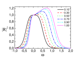
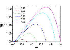
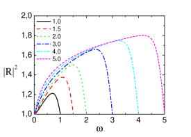
Figure 6: Reflection coefficient $\left|R_{\omega m}\right|^{2}$ as a function of $\omega$ for $m=1$. Each curve corresponds to a different value of $B$, as indicated. The top panels show that the reflection coefficient decays exponentially at the critical frequency for superradiance, $\omega_{SR}=mB$. The middle panels show a close-up view in the superradiant regime for $B<1$: at $B=1$ the maximum amplification is 21.2 %. The bottom panels show that superradiant amplification can become much more efficient for values of the rotation parameter $B>1$.

Results of the numerical integrations for the draining bathtub metric are shown in Fig. 6. Panels on the left show the reflection coefficient $|R_{\omega 1}|^{2}$ for $m=1$, and panels on the right show $|R_{\omega 2}|^{2}$ for $m=2$, for selected values of the black hole rotation $B$. Panels on top show that, as expected, in the superradiant regime $0<\omega<mB$ the reflection coefficient $|R_{\omega m}|^{2}\geq 1$. Furthermore, as one increases $B$ the reflection coefficient increases, and for fixed $B$, the reflection coefficient $\left|R_{\omega m}\right|^{2}$ attains a maximum at $\omega\sim mB$, after which it decays exponentially as a function of $\omega$ outside the superradiant interval. This is very similar to what happens when one deals with massless fields in the vicinities of rotating Kerr black holes teupress . In particular, from the close-up view in the middle panels we see that, for $B=1$, the maximum amplification is 21.2 % ($m=1$) and 4.7 % ($m=2$).

As a final remark, and as we have anticipated, an important difference between the acoustic black hole metric and the Kerr metric is that in the present case there is no mathematical upper limit on the black hole’s rotational velocity $B$. In the bottom panels we show that, considering values of $B>1$, we can indeed have larger amplification factors for acoustic black holes.

Summarizing: if we are clever enough to build in the lab an acoustic black hole that spins very rapidly, rotational superradiance can be particularly efficient in analogues. This is an important result, considering that the detection of rotational superradiance in the lab is by no means an easy task, as originally predicted by Zel’dovich zel and confirmed by recent reconsideration of the problem bekenstein . Of course, in any real-world experiment the maximum rotational parameter will be limited. At the mathematical level, the equations describing sound propagation (which are written assuming the hydrodynamic approximation) will eventually break down. Physically, if the angular component of the velocity $v^{\theta}$ becomes very large the dispersion relation for the fluid will change, invalidating the assumptions under which we have derived our acoustic metric schutzhold ; waveanalog1 .

The superradiant phenomena we have described are purely classical in nature. However, an interesting suggestion to observe quantum effects in acoustic superradiance was put forward in basak2 . To write down our acoustic metric we required the flow to be irrotational and non-viscous. As a natural choice, we could use a fluid which is well known to possess precisely these properties: superfluid HeII. In this case the presence of vortices with quantized angular momenta may lead to a quantized energy flux. The heuristic argument presented in basak2 goes as follows. Let us imagine that our black hole is a vortex with a sink at the center. In the quantum theory of HeII the wavefunction is of the form $\Psi=\exp\left[{\rm i}\sum_{j}\phi(\vec{r}_{j})\Phi_{\rm ground}\right]$, where $\vec{r}_{j}$ is the position of the $j$-th particle of HeII. The velocity at any point is given by the gradient of the phase at that point, $\vec{v}=\nabla\phi$, so that (roughly speaking) the velocity potential can be identified with the phase of the wavefunction. This phase will be singular at the sink $r=0$. Continuity of the phase around a circle surrounding the sink requires that the change of the wavefunction satisfies $\Delta\phi=2\pi B$. For the wavefunction to be single valued, $B$ (that is, the black hole’s angular velocity at the horizon) must be the integer multiple of some minimum value $\Delta B$, i.e., $B=n\,\Delta B$. Then the angular momentum of the acoustic black hole would be forced to change in integer multiples of $\Delta B$. Correspondingly, the spectrum of the reflection coefficients may be given by equally-spaced peaks with different strengths. This discrete amplification could enhance chances of observing superradiance in acoustic black holes, and rule out (or provide empirical support to) some of the many competing heuristic approaches to black hole quantization.

IV.4 Acoustic black branes and superradiant instabilities

Now, we are free to add an extra dimension and interpreting the result as the superposition of a vortex filament and a line sink visser . We get therefore the following line element

$$ds^{2} = -\left(1-\frac{A^{2}+B^{2}}{c^{2}r^{2}}\right)c^{2}d\tilde{t}^{2}+\left(1-\frac{A^{2}}{c^{2}r^{2}}\right)^{-1}dr^{2}-$$ (45)

$$2Bd\tilde{\phi}d\tilde{t}+r^{2}d\tilde{\phi}^{2}+dz^{2}\,.$$

This describes an analogue black brane, and compactification of the transverse direction $z$ can be accomplished, in practice by using a “tamper” around the flow.

The propagation of a sound wave in a barotropic inviscid fluid with irrotational flow is described by the Klein-Gordon equation $\nabla_{\mu}\nabla^{\mu}\Psi=0$ for a massless field $\Psi$ in a Lorentzian acoustic geometry, which in our case takes the form (45). In our acoustic geometry we can separate variables by the substitution

$$\Psi(\tilde{t},r,\tilde{\phi})=\frac{1}{\sqrt{r}}H(r)e^{{\rm i}(m\tilde{\phi}+\mu z-\omega\tilde{t})}\,,$$ (46)

and we get the wave equation

$$H_{,r_{*}r_{*}}+\left\{\left(\omega-\frac{Bm}{r^{2}}\right)^{2}-V\right\}H=0$$ (47)

$$V=f\left[\frac{1}{r^{2}}\left(m^{2}-\frac{1}{4}\right)+\frac{5}{4r^{4}}+\mu^{2}\right]\,.$$ (48)

To arrive at (48) we have already performed the following re-scaling: $\hat{r}=rA/c$, $\hat{\omega}=\omega A/c^{2}$, $\hat{B}=B/A$, $\hat{\mu}=\mu c/A$. The re-scaling effectively sets $A=c=1$ in the original wave equation, and picks units such that the acoustic horizon $\hat{r}_{H}=1$. The quantity $f\equiv(1-\frac{A^{2}}{c^{2}r^{2}})$, and the tortoise coordinate $r_{*}$ is defined by the condition

$$\frac{dr_{*}}{dr}=\frac{1}{f}\,.$$ (49)

Explicitly,

$$r_{*}=r+\frac{A}{2c}\log\left|\frac{cr-A}{cr+A}\right|\,.$$ (50)

It is known that the Kerr geometry, or any rotating (absorbing) body displays superradiance zel ; misnerunruhbekenstein . This means that in a scattering experiment of a wave with frequency $\omega<m\Omega$ the scattered wave will have a larger amplitude than the incident wave, the excess energy being withdrawn from the object’s rotational energy. Here $\Omega$ is the horizon’s angular velocity and $m$ is an azimuthal quantum number. Now suppose that one encloses the rotating black hole in a spherical mirror. Any initial perturbation will get successively amplified near the black hole event horizon and reflected back at the mirror, thus creating an instability. This is the black hole bomb, as devised in teupress and recently improved in bhb . This instability is caused by the mirror, which is an artificial wall, but one can devise “natural mirrors” if one considers massive fields. Imagine a wavepacket of the massive field in a distant circular orbit. The gravitational force binds the field and keeps it from escaping or radiating away to infinity. But at the event horizon some of the field goes down the black hole, and if the frequency of the field is in the superradiant region then the field is amplified. Hence the field is amplified at the event horizon while being bound away from infinity. Yet another way to understand this, is to think in terms of wave propagation in an effective potential. If the effective potential has a well, then waves get “trapped” in the well and amplified by superradiance, thus triggering an instability. In the case of massive fields on a (four-dimensional) Kerr background, the effective potential indeed has a well, as we show in Figure 7. Consequently, the massive field grows exponentially and is unstable (see schwinger ; detweiler ; zouros ; furu ; braneinstability for explicit examples).

Figure 7: A typical form for the effective potential in the Kerr geometry, here shown for $l=m=1$ modes. We have set the mass of the black hole $M=1$, so the rotation parameter $a$ varies between $0$ (Schwarzschild limit) and $1/2$ (extremal limit). Here we plot the effective potential for the near extreme situation, $a\sim 0.5$ and for $\mu=0.7$ and $\omega=0.6878$.

With this in mind, we would expect that black strings and branes of the form (45) for which there is a bound state will be unstable; here the transverse direction $z$ works as an effective mass for the sound wave. To get a bound state, one necessary condition is that the derivative of the potential is positive, at asymptotic large radial distances (see braneinstability for more details). Now, near infinity, we get

$$V_{eff}\sim\frac{4m^{2}-1-\mu^{2}+8\omega mB}{4r^{2}}\,,$$ (51)

which leads to

$$V^{\prime}_{eff}\sim\frac{4\mu^{2}+1-4m^{2}-8\omega mB}{2r^{3}}\,.$$ (52)

Now, this can be positive, thus an instability can be triggered.

For the sake of generality, let us drop the constant $\rho$ requirement, which means not assuming conservation of angular momentum (this can be achieved by having external torques), then we can show that the effective metric is

$$ds^{2}\!\! = \!\!-\left(1-\frac{A^{2}/\rho^{2}+B^{2}}{c^{2}r^{2}}\right)c^{2}d\tilde{t}^{2}$$

$$+\left(1-\frac{A^{2}}{\rho^{2}c^{2}r^{2}}\right)^{-1}dr^{2}-2Bd\tilde{\phi}d\tilde{t}+r^{2}d\tilde{\phi}^{2}+dz^{2}\,.$$

Here, $A\,,B$ are again constants but they have different dimensions. Separating variables by the substitution

$$\Phi(\tilde{t},r,\tilde{\phi})=\sqrt{r}\Psi(r)e^{i(\mu z+m\tilde{\phi}-\omega\tilde{t})}\,,$$ (54)

implies that $\Psi(r)$ obeys the wave equation (just insert the ansatz in Klein-Gordon’s equation)

$$\frac{d^{2}\Psi}{dr_{*}^{2}}+\left((\omega-\frac{Bm}{r^{2}})^{2}-V\right)\Psi=0\,.$$ (55)

Here

$$V = f\left(\mu^{2}c+\frac{4m^{2}c-c}{4r^{2}}+\frac{c^{\prime}}{2r}\right)+$$ (56)

$$f\left(\frac{A^{2}}{4cr^{4}\rho^{2}}\left(5+2r(\frac{c^{\prime}}{c}+\frac{2\rho^{\prime}}{\rho})\right)\right)\,,$$

and the tortoise coordinate $r_{*}$ is defined as

$$\frac{dr}{dr_{*}}=c(1-\frac{A^{2}}{c^{2}\rho^{2}r^{2}})\equiv f\,.$$ (57)

Notice that for constant $\rho\,,\,c$ one recovers the equations (48), as one should. Now, it is quite easy to present an example flow which the instability is triggered: take for instance a flow for which $\rho$ is almost constant at infinity (almost means that it asymptotes to a constant value more rapidly than the sound velocity). Assume also that, near infinity, $c=c_{1}+\frac{c_{2}}{r}$. Then, we get that near infinity the effective potential behaves as

$$\frac{2c_{1}c_{2}k^{2}}{r}\,.$$ (58)

For this to have a positive derivative, one requires $c_{2}<0$ ($c_{1}$ must be positive, as it is the asymptotic value of the sound velocity). We thus have one example of flow for which the instability is active. There are many others, of course, and there are also instances for which the system is stable.

IV.5 Absorption cross-sections

The computation of absorption cross-sections may be handled analytically in the low frequency regime, to which I now turn. The computation of absorption cross-sections of different gravitational black holes has gained a special interest some years ago, since it was shown that string theory could reproduce these results (for some particular geometries). I refer the reader to oz for a introduction to the subject. Considering again our ($2+1$)-dimensional rotating acoustic black hole we shall now attempt at solving the wave equation in this geometry, in the limit of small $\omega$. The method we use here follows closely the work of Starobinsky and Churilov superr and Unruh and others cross . The wave equation reads waveanalog1 :

$$H_{,r_{*}r_{*}}+\left\{\left(\omega-\frac{Bm}{r^{2}}\right)^{2}-V\right\}H=0$$ (59)

$$V=f\left[\frac{1}{r^{2}}\left(m^{2}-\frac{1}{4}\right)+\frac{5}{4r^{4}}\right]\,.$$ (60)

The computation will follow closely that in cardosodias . Changing wavefunction to $R=r^{-1/2}H$ we find that $R$ satisfies

$$\Delta\partial_{r}\left(\Delta\partial_{r}R\right)+\left(\omega^{2}r^{2}-2Bm\omega+\frac{B^{2}m^{2}}{r^{2}}-\frac{\Delta m^{2}}{r}\right)R=0\,,$$ (61)

where $\Delta=r-1/r$. Let us solve this equation in the far-region, $r>>1$. We then have, near infinity,

$$\Delta\partial_{r}\left(\Delta\partial_{r}R\right)\sim r^{2}\partial^{2}_{r}R+r\partial_{r}R\,.$$ (62)

Assuming $B\omega<<1$, the wave equation (61) in this region takes the form

$$r^{2}\partial^{2}_{r}R+r\partial_{r}R+\left(\omega^{2}r^{2}-m^{2}\right)R=0\,.$$ (63)

Defining $\rho=\omega r$ this takes the form

$$\rho^{2}\partial^{2}_{\rho}R+\rho\partial_{\rho}R+\left(\rho^{2}-m^{2}\right)R=0\,,$$ (64)

which is a Bessel equation (see for example abramowitz ; niki ), with the general solution

$$R=\alpha J_{m}(\omega r)+\beta Y_{m}(\omega r)\,.$$ (65)

Notice that $m$ is an integer, and therefore $J_{m}$ and $J_{-m}$ are not linearly independent.

We will want later on to do a matching between the near region solution and the far-region solution, so let us investigate the near region behavior of this solution, or the limit $\omega r\rightarrow 0$. We find cardosodias

$$R\sim\frac{\alpha}{\Gamma[m+1]}(\frac{\omega r}{2})^{m}-\frac{\beta}{\pi}\Gamma[m](\frac{\omega r}{2})^{-m}\,,$$ (66)

where $\psi$ is the digamma function. We now define the near-region as the range for which $r-r_{+}<<\frac{1}{\omega}$. Defining

$$z=\frac{r_{+}}{r^{2}}$$ (67)

$$R=z^{\alpha}(1-z)^{\beta}T\,,$$ (68)

then, in this region the solution representing ingoing waves at the horizon (which is the boundary condition one must impose) may be written as cardosodias

$$T=A_{1}F[a,b,a+b-c+1,1-z]\,,$$ (69)

where

$$a=1+\frac{m}{2}-i\varpi\,,$$ (70)

$$b=\frac{m}{2}-i\varpi\,,$$ (71)

$$c=1+m\,.$$ (72)

Here $\varpi\equiv\frac{\omega-mB}{2}$, and $F[.,.,.,]$ denotes the standard hypergeometric functions. Since $c=m+1$ is a integer, one must be very careful in handling the hypergeometric function abramowitz ; niki .

When $z\rightarrow 0$, or $r\rightarrow\infty$, we have

$$R\sim Ar^{-m}\{\psi(a)+\psi(b)-\psi(1+m)-\psi(1)\}+$$

$$Ar^{m}\{\frac{(-1)^{m-1}\Gamma[m]}{m!(a-m)_{m}(b-m)_{m}}\}\,,$$ (73)

where $A$ is some constant and $(a)_{m}$ stands for $(a)_{m}=a(a+1)(a+2)...(a+m-1)\,,(a_{0})=1$. Matching the two solutions (66) and (73) we get

$$\frac{\alpha}{\beta}=\frac{1}{\pi}\frac{(-1)^{m}\Gamma[m]^{2}(\omega/2)^{-2m}}{(a-m)_{m}(b-m)_{m}(\psi(a)+\psi(b)-\psi(m+1)-\psi(1))}\,.$$ (74)

Now, $(a-m)_{m}=\frac{\Gamma[a]}{\Gamma[a-m]}$, we thus have

$$\frac{\alpha}{\beta}=\frac{1}{\pi}\frac{(-1)^{m}\Gamma[m]^{2}\Gamma[a-m]\Gamma[b-m](\omega/2)^{-2m}}{\Gamma[a]\Gamma[b](\psi(a)+\psi(b)-\psi(m+1)-\psi(1))}\,.$$ (75)

This is the final expression. Since $\alpha,\beta$ are related to the amplitude of in- and out-going waves at infinity, using (75) we can straightforwardly compute reflection coefficients, absorption cross sections, etc.

V Conclusions

Analogue black holes have proven to be a very valuable tool for the investigation of problems related to Hawking radiation. It is also possible that will yield valuable information regarding classical phenomena involving black holes. We have shown here some aspects of classical phenomena involving acoustic black holes, that may prove useful for future experimental realization of these systems.

References

- (1) S. Chandrasekhar, in The Mathematical Theory of Black Holes, (Oxford University Press, New York, 1983).
- (2) B. Carter and R. Ruffini, in Black Holes: les Astres Occlus, (Gordon and Breach Science Publishers, 1973); B. Carter, in Black Hole Physics(NATO ASI C364), eds. V. de Sabbata, Z. Zhang (Kluwer, Dordrecht, 1992) 283-357; hep-th/0411259.
- (3) S. L. Shapiro and S. A. Teukolsky, in Black Holes, White Dwarfs and Neutron Stars: The Physics of Compact Objects, (John Wiley and Sons, New York, 1983).
- (4) P. Anninos, D. Hobill, E. Seidel, L. Smarr and W-M Suen, Phys. Rev. Lett. 71, 2851 (1993); P. Anninos and S. Brandt, Phys. Rev. Lett. 81, 508 (1998).
- (5) S. W. Hawking, Nature 248, 30 (1974); S. W. Hawking, Commun. Math. Phys. 43, 199 (1975).
- (6) A. Strominger and C. Vafa, Phys. Lett. B 379, 99 (1996).
- (7) B. Zwiebach, in A First Course in String Theory, (Cambridge University Press, Cambridge, 2004).
- (8) O. Aharony, S. Gubser, J. Maldacena, H. Ooguri and Y. Oz, Phys. Reports 323, 183 (2000).
- (9) J. Maldacena, Black Holes in String Theory, PhD thesis (unpublished); hep-th/9607235.
- (10) W. G. Unruh, Phys. Rev. Lett. 46, 1351 (1981).
- (11) M. Visser, Class. Quantum Grav. 15, 1767 (1998).
- (12) M. Novello, M. Visser and G. Volovik (editors), Artificial black holes (World Scientific, Singapore, 2002).
- (13) T. K. Das, gr-qc/0411006.
- (14) M. Visser, Int. J. Mod. Phys. D 12, 649 (2003).
- (15) R. Schutzhold and W. G. Unruh, quant-ph/0408145.
- (16) J. A. H. Futterman, F. A. Handler and R. A. Matzner, in Scattering From Black Holes, (Cambridge University Press, Cambridge, 1988).
- (17) Ya. B. Zel’dovich, Pis’ma Zh. Eksp. Teor. Fiz. 14, 270 (1971) [JETP Lett. 14, 180 (1971)]; Zh. Eksp. Teor. Fiz 62, 2076 (1972) [Sov. Phys. JETP 35, 1085 (1972)].
- (18) W. Israel, in 300 Years of Gravitation, edited by S. W. Hawking & W. Israel (Cambridge University Press, Cambridge 1987) pgs. 199–276.
- (19) J. D. Bekenstein and M. Schiffer, Phys. Rev. D 58, 064014 (1998).
- (20) E. Berti, V. Cardoso and J. P. S. Lemos, Phys. Rev. D 70, 124006 (2004).
- (21) V. Cardoso, J. P. S. Lemos and S. Yoshida, Phys. Rev. D 70, 124032 (2004).
- (22) T.R. Slatyer and C.M. Savage, cond-mat/0501182.
- (23) K. D. Kokkotas and B. G. Schmidt, Living Rev. Rel. 2, 2 (1999); H.-P. Nollert, Class. Quantum Grav. 16, R159 (1999).
- (24) V. Cardoso, “ Quasinormal Modes and Gravitational Radiation in Black Hole Spacetimes”, PhD thesis, Instituto Superior Tecnico, Universidade Técnica de Lisboa, December 2003, gr-qc/0404093.
- (25) V. Cardoso, J. P. S. Lemos and S. Yoshida, Phys. Rev. D 69, 044004 (2004); E. Berti, V. Cardoso, K. Kokkotas and H. Onozawa, Phys. Rev. D 68, 124018 (2003); E. Berti, V. Cardoso and S. Yoshida, Phys. Rev. D 69, 124018; V. Cardoso, J. Natário and R. Schiappa, J. Math. Phys. 45, 4698 (2004); V. Cardoso, Ó. J. C. Dias, J. P. S. Lemos, Phys. Rev. D 67, 064026 (2003); E. Berti and K. D. Kokkotas, gr-qc/0502065.
- (26) H. Nakano, Y. Kurita, K. Ogawa and C.-M. Yoo, Phys. Rev. D 71, 084006 (2005); S. Lepe and J. Saavedra, gr-qc/0410074.
- (27) R. H. Price, Phys. Rev. D5, 2419 (1972); E. S. C. Ching, P. T. Leung, W. M. Suen and K. Young, Phys. Rev. Lett. 74, 2414 (1995); E. S. C. Ching, P. T. Leung, W. M. Suen and K. Young, Phys. Rev. D 52, 2118 (1995); V. Cardoso, S. Yoshida, O. J. C. Dias, J. P. S. Lemos, Phys. Rev. D 68, 061503 (2003).
- (28) R. D. Blandford and R. L. Znajek, Mon. Not. Roy. Astron. Soc. 179, 443 (1977).
- (29) D. R. Sisan at al, Phys. Rev. Lett 93, 114502 (2004).
- (30) S. Corley and T. Jacobson, Phys. Rev. D 59, 124011 (1999).
- (31) T. Damour, N. Deruelle and R. Ruffini, Lett. Nuovo Cim. 15, 257 (1976).
- (32) S. Detweiler, Phys. Rev. D 22, 2323 (1980).
- (33) T. M. Zouros and D. M. Eardley, Annals of Physics 118, 139 (1979).
- (34) H. Furuhashi and Y. Nambu, gr-qc/0402037; M. J. Strafuss and G. Khanna, gr-qc/0412023.
- (35) S. Hod, Phys. Rev. Lett. 81, 4293 (1998).
- (36) M. Visser, Phys. Rev. Lett. 80, 3436 (1998).
- (37) M. Cadoni, Class. Quantum Grav. 22, 409 (2005).
- (38) R. Schützhold, W. G. Unruh, Phys. Rev. D 66, 044019 (2002).
- (39) V. Cardoso and J. P. S. Lemos, hep-th/0412078; V. Cardoso and S. Yoshida, hep-th/0502206.
- (40) L. Landau and E. Lifshitz, Fluid dynamics (Mir, Moscow, 1974).
- (41) A. H. Shapiro, in Compressible Fluid Flow, (The Ronald Press Company, New York, 1953);
- (42) S. Chandrasekhar, Hydrodynamic and Hydromagnetic Stability (Dover Publications, New York, 1981).
- (43) C. Barcelo, S. Liberati and M. Visser, Int. J. Mod. Phys. A 18, 3735 (2003) 3735.
- (44) S. Liberati, S. Sonego and M. Visser, Class. Quantum Grav. 17, 2903 (2000).
- (45) P. Painlevé, C. R. Hebd. Seances Acad. Sci. 173, 677 (1921); A. Gullstrand, Ark. Mat. Astron. Fys. 16, 1 (1922); G. Lemaître, Ann. Soc. Sci. Bruxelles, Ser. 1 53, 51 (1933).
- (46) J. Bekenstein, in Cosmology and Gravitation, edited by M. Novello (Atlasciences, France 2000), pp. 1-85; gr-qc/9808028 (1998).
- (47) For recent developments relating quasinormal modes with decay timescales in the AdS/CFT see G. T. Horowitz and V. E. Hubeny Phys. Rev. D 62, 024027 (2000); B. Wang, C. Y. Lin, and E. Abdalla, Phys. Lett. B 481, 79(2000); B. Wang, C. M. Mendes, and E. Abdalla, Phys. Rev. D 63, 084001(2001). V. Cardoso and J. P. S. Lemos, Phys. Rev. D63, 124015 (2001); Phys. Rev. D 64, 084017 (2001); Phys. Rev. D 66, 064006 (2002); R. A. Konoplya, Phys. Rev. D66, 044009 (2002); E. Berti and K.D. Kokkotas, Phys. Rev. D67, 064020 (2003); V. Cardoso, R. Konoplya and J. P. S. Lemos, Phys. Rev. D 68, 044024 (2003).
- (48) S. Hassani, Mathematical Physics, (Springer-Verlag, New York, 1998); R. Courant and D. Hilbert, Methods of Mathematical Physics, Chapter VI (Interscience, New York, 1962).
- (49) H. Soodak and M. S. Tiersten, Am. J. Phys. 61, 395 (1993).
- (50) V. L. Ginzburg and I. M. Frank, Dokl. Akad. Nauk SSSR 56, 583 (1947); for a recent review cf. V. L. Ginzburg, in Progress in Optics XXXII, edited by E. Wolf (Elsevier, Amsterdam, 1993).
- (51) C. W. Misner, Phys. Rev. Lett. 28, 994 (1972); A. A. Starobinsky, Sov. Phys. JETP 37, 28 (1973); A. A. Starobinsky and S. M. Churilov, Sov. Phys. JETP 38, 1 (1973); W. Unruh, Phys. Rev. D 10, 3194 (1974); W. H. Press and S. A. Teukolsky, Astrophys. Journal 185, 649 (1973).
- (52) W. H. Press and S. A. Teukolsky, Nature 238, 211 (1972).
- (53) J. D. Bekenstein, Phys. Rev. D 7, 949 (1973).
- (54) R. Penrose, Nuovo Cimento 1, 252 (1969).
- (55) J. L. Friedman, Commun. Math. Phys. 63, 243 (1978).
- (56) N. Comins and B. F. Schutz, Proc. R. Soc. Lond. A 364, 211 (1978).
- (57) S. Yoshida and E. Eriguchi, MNRAS 282, 580 (1996).
- (58) V. Cardoso, O. J. C. Dias, J. P. S. Lemos and S. Yoshida, Phys. Rev. D 70, 044039 (2004); V. Cardoso and O. J. C. Dias, Phys. Rev. D 70, 084011 (2004).
- (59) S. Basak and P. Majumdar, Class. Quant. Grav. 20, 2929 (2003).
- (60) S. Basak and P. Majumdar, Class. Quant. Grav. 20, 3907 (2003).
- (61) T. Jacobson and G. E. Volovik, Phys. Rev. D 58, 064021 (1998).
- (62) C. W. Misner, Phys. Rev. Lett. 28, 994 (1972); J. Bekenstein Phys. Rev. D 7, 949 (1973); W. Unruh, Phys. Rev. D 10, 3194 (1974).
- (63) V. Cardoso and O. J. C. Dias, unpublished.
- (64) M. Abramowitz and A. Stegun, Handbook of mathematical functions (Dover Publications, New York, 1970).
- (65) A. F. Nikiforov, V. B. Uvarov, Special Functions of Mathematical Physics, (Birkhäuser, Boston, 1988).
- (66) W. G. Unruh, Phys. Rev. D 14, 3251 (1976); J. M. Maldacena and A. Strominger, Phys. Rev. D 56, 4975 (1997).