Inference of a nonlinear stochastic model of the cardiorespiratory interaction

Abstract

A new technique is introduced to reconstruct a nonlinear stochastic model of the cardiorespiratory interaction. Its inferential framework uses a set of polynomial basis functions representing the nonlinear force governing the system oscillations. The strength and direction of coupling, and the noise intensity are simultaneously inferred from a univariate blood pressure signal, monitored in a clinical environment. The technique does not require extensive global optimization and it is applicable to a wide range of complex dynamical systems subject to noise.

Heart rate variability (HRV) is an important dynamical phenomenon in physiology. Altered HRV is associated with a range of cardiovascular diseases and increased mortality Camm:96 , and its parameters are starting to be used as a basis for diagnostic tests. However, signals acquired from the human cardiovascular system (CVS), being derived from a living organism, arise through the interaction of many dynamical degrees of freedom and processes with different time scales Winfree:80Glass:88 . Thus HRV is attributable to the mutual interaction of a large number of oscillatory processes. Among them, the effect of respiration on heart rate has been the most intensively studied. The physiological mechanisms have recently been reviewed Eckberg:03 and include e.g. modulation of the cardiac filling pressure as a result of changes of intrathoracic pressure during respiratory movements Visscher:24 , direct respiratory ordering of autonomic outflow Eckberg:03 , and baroreceptor feedback control deBoer:87 .

An important feature of these processes is that they are nonlinear, time-varying, and subject to fluctuations  Saul:88a ; Chon:96Suder:98 ; Stefanovska:99a . For such systems deterministic techniques fail to yield accurate parameter estimates Kostelich:92McSharry:99a . Additionally, models of the cardiovascular interactions are not usually known exactly from first principles and one is faced with a rather broad range of possible parametric models to consider  deBoer:87 ; Clynes:60Baselli:88TenVoorde:95Seidel:95Cavalcanti:96Kotani:02 . Inverse approaches, in which dynamical properties are analysed from measured data have recently been considered. A variety of numerical techniques have been introduced to analyse cardio-respiratory interactions using e.g. linear approximations Berger:89Taylor:01Mukkamala:01Chon:01b , estimations of either the strength of some of the nonlinear terms Jamsek:03Jamsek:04 , the occurrence of cardio-respiratory synchronization Schaefer:98Janson:01 or the directionality of coupling Rosenblum:02Palus:03a . Hitherto, modelling approaches have not been used interactively in conjunction with time series analysis methods. Rather, the latter have each focussed on a particular dynamical property, e.g. synchronization, or nonlinearities, or directionality.

In this Letter we introduce an approach to the problem that combines mathematical modelling of system dynamics and extraction of model parameters directly from measured time series. In this way we estimate simultaneously the strength, directionality of coupling and noise intensity in the cardio-respiratory interaction. The technique reconstructs the nonlinear system dynamics in the presence of fluctuations. In addition, the method provides optimal compensation of dynamical noise-induced errors for continuous systems while avoiding extensive numerical optimization. We demonstrate the approach by using a univariate blood pressure (BP) signal for reconstruction of a nonlinear stochastic model of the cardio-respiratory interaction. The results are verified by analysis of data synthesized from the inferred model.

The problems faced in the analysis of CVS variability are common, not only to all living systems, but also to all complex systems subject to fluctuations, e.g. molecular motors Visscher:99 or coupled matter–radiation systems in astrophysics Christensen:02 . Yet there are no general methods for the dynamical inference of stochastic nonlinear systems. Thus the technique introduced in this paper will be of wide applicability.

We use public domain data to illustrate the idea. We analyse central venous blood pressure data, record 24 of the MGH/MF Waveform Database available at www.physionet.org. Its spectrum, shown in Fig. 1(a), exhibits two basic frequencies corresponding to the respiratory, $f_{r}\approx 0.2$ Hz, and cardiac, $f_{c}\approx 1.7$ Hz, oscillations; the higher frequency peaks are the 2nd, 3rd and 4th harmonics of the cardiac oscillation. We note that the relative intensity and position of these peaks vary from subject to subject, with the average frequencies for healthy subjects at rest being around $0.2$ and $1.1$ Hz for respiration and heart rate respectively.

We must bear in mind that CVS power spectra also contain lower frequency components Camm:96 ; Stefanovska:97aTaylor:98Stefanovska:01b . In practice, parametric modelling is usually restricted to a specific part of the power spectrum. Because our interest here centres on the cardio-respiratory interaction, we select for study the frequency range that includes the main harmonics of cardiac and respiratory oscillations $f_{c}$ and $f_{r}$ and their combinational frequencies as shown in Fig. 1(b). In addition, we assume that the two higher basic frequency components observed in all CVS signals Stefanovska:99a ; Stefanovska:01a can be separated. Hence the blood pressure signal can be considered in the first approximation as a sum of the cardiac and respiratory oscillatory components $s(t)=s_{c}(t)+s_{r}(t)$. Accordingly, we use a combination of zero-phase forward and reverse digital filtering based on Butterworth filters to decompose Decomposition the blood pressure signal into 2-dimensional time series $\{{\bf s}(t_{k})=(s_{c}(t_{k}),s_{r}(t_{k})),\,\,t_{k}=kh,\,k=0:K\}$. The time series represent the contributions of cardiac and respiratory oscillations to the blood pressure on a discrete time grid. A window consisting of 18000 points of the original signal, sampled at 360 Hz, was resampled at 90 Hz. Hence the signal considered for inference was of length 500 s, with a step size of $h=1/90$ sec.

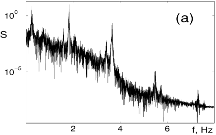
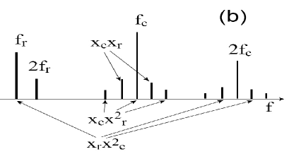
Figure 1: (a) Power spectrum of the venous blood pressure (BP) data after filtration through Butterworth filters: low-pass of the 4^th order, with a cut-off frequency of 3 Hz; and high-pass of the 2^nd order with cut-off frequency of 0.03 Hz. (b) Summary of the main combinatorial frequencies of the cardiac and respiratory components observed in the BP signal. The correspondence between the nonlinear interaction terms of the model (3) and the frequencies observed in the time-series data are shown by arrows.

Following the suggestion of coupled oscillators Stefanovska:99a ; Stefanovska:01a , we now choose the simplest model that can reproduce this type of oscillation: two nonlinearly coupled systems with limit cycles on a plane

$$\left\{\begin{array}[]{ll}\dot{x}_{r}=a_{1}x_{r}+y_{r},&\dot{y}_{r}=\alpha_{i}\phi_{i}({\bf x},{\bf y})+\sqrt{D_{1j}}\xi_{j},\\ \dot{x}_{c}=a_{2}x_{c}+y_{c},&\dot{y}_{c}=\beta_{i}\phi_{i}({\bf x},{\bf y})+\sqrt{D_{2j}}\xi_{j}\end{array}\right.$$ (3)

are included. Here $\xi_{j}(t)$ are zero-mean white Gaussian noises, and the summation is taken over repeated indexes $i=1,...,22$ and $j=r,c$. The base functions are chosen in the form

$$\phi=\{1,x_{r},x_{c},y_{r},y_{c},x_{r}^{2},x_{c}^{2},y_{r}^{2},y_{c}^{2},x_{r}y_{r},x_{c}y_{c},x_{r}^{3},$$

$$x_{c}^{3},x_{r}^{2}y_{r},x_{c}^{2}y_{c},x_{r}y_{r}^{2},x_{c}y_{c}^{2},y_{r}^{3},y_{c}^{3},x_{r}x_{c},x_{r}^{2}x_{c},x_{r}x_{c}^{2}\},$$ (4)

that includes nonlinear coupling terms up to 3rd order. We assume that the measurement noise can be neglected. The two dynamical variables of the model (3), $x_{r}(t)$ and $x_{c}(t)$ correspond to the two-dimensional time-series, ${\bf s}(t)=\{s_{r}(t),s_{c}(t)\}$, introduced above. Using (3) the remaining two dynamical variables ${\bf y}(t)=\{y_{r}(t),y_{c}(t)\}$ can be related to the observations $\{{\bf s}(t_{k})\}$ as follows

$$b_{n}y_{n}(t_{k})=\frac{s_{n}(t_{k}+h)-s_{n}(t_{k}-h)}{2h}+a_{n}s_{n}(t_{k}),$$ (5)

where $n=r,c$. Parametric presentation (3) with a special form of embedding (5) allows one to infer a wide class of dynamical models including e.g. the van der Pol and FitzHugh-Nagumo models. Furthermore, it allows physiological interpretation of the model parameters.

Using (5) we can reduce the original problem of characterizing the cardio-respiratory interaction to that of inferring the set of unknown parameters ${\cal M}=\{{\bf c},{\bf\hat{D}}\}$ of the coupled stochastic nonlinear differential equations

$$\dot{\bf y}={\bf\hat{U}}({\bf s},{\bf y}){\bf c}+\sqrt{\bf\hat{D}}{\bm{\xi}}(t).$$ (6)

Here ${\bm{\xi}}(t)$ is a two-dimensional Gaussian white noise with independent components mixed with unknown correlation matrix ${\bf\hat{D}}$. The matrix ${\hat{\bf U}}$ will have the following block structure

$${\hat{\bf U}}=\left[\left[\begin{array}[]{ll}1&0\\ 0&1\\ \end{array}\right],\left[\begin{array}[]{ll}x_{r}&0\\ 0&x_{r}\\ \end{array}\right]\ldots\left[\begin{array}[]{ll}x_{r}x_{c}^{2}&0\\ 0&x_{r}x_{c}^{2}\\ \end{array}\right]\right].$$ (13)

The vector of unknown coefficients ${\bf c}=\{\alpha_{1},\beta_{1},...,\alpha_{22},\beta_{22}\}$ has the length $M=2B$, where $B=22$ diagonal blocks of size $2\times 2$ formed by the basis functions (Inference of a nonlinear stochastic model of the cardiorespiratory interaction).

The model parameters can be obtained by use of our novel method of dynamical inference of stochastic nonlinear models. The method is based on the Bayesian technique. Details, and a comparison with the results of earlier research, are given elsewhere Smelyanskiy:submitted . Here we describe briefly the main steps in applying the method to inference of cardio-respiratory interactions. First, one has to define the so-called likelihood function $\ell({\bf y}|{\cal M})$: the probability density to observe the dynamical variables ${\bf y}(t)$ under the condition that the underlying dynamical model (6) has a given set of parameters ${\cal M}$. We suggest that, for a uniform sampling scheme and a sufficiently small time step $h$, one can use results from Graham:77 to write the logarithm of the likelihood function as

$$-\frac{2}{K}\log\ell({\bf y}|{\cal M})=\ln\det{\hat{\bf D}}+\frac{h}{K}\sum_{k=0}^{K-1}\left[\,{\bf v}({\bf y}_{k}){\bf c}\right.$$ (14)

$$\left.+(\dot{\bf y}_{k}-{\hat{\bf U}}_{k}\,{\bf c})^{T}\,{\hat{\bf D}}^{-1}\,(\dot{\bf y}_{k}-{\hat{\bf U}}_{k}\,{\bf c}))\right]+N\ln(2\pi h).$$

Here ${\bf\hat{U}}_{k}\equiv{\bf\hat{U}}({\bf y}_{k})$, $\dot{\bf y}_{k}\equiv h^{-1}({\bf y}_{k+1}-{\bf y}_{k})$ and the vector ${\bf v}({\bf x})$ has components

$$\textrm{v}_{m}({\bf x})=\sum_{n=1}^{N}\frac{\partial U_{n\,m}({\bf x})}{\partial x_{n}},\quad m=1:M.$$

Note that the form of (14) differs from the cost function in the method of least-squares: the term involving ${\bf v}$ provides optimal compensation of noise-induced errors  Smelyanskiy:submitted . In the next step one has to summarize a priori expert knowledge about the model parameters in the so-called prior PDF, $p_{\textrm{pr}}({\cal M})$. We assume $p_{\textrm{pr}}({\cal M})$ to be Gaussian with respect to the elements of ${\bf c}$ and uniform with respect to the elements of ${\bf\hat{D}}$.

Finally, one can use the measured time-series ${\bf y}$ to improve the a priori estimation of the model parameters. The improved knowledge is summarized in the posterior conditional PDF $p_{\textrm{post}}({\cal M}|{\bf y})$, which is related to the prior PDF via Bayes’ theorem

$$p_{\textrm{post}}({\cal M}|{\bf y})=\frac{{\ell}({\bf y}|{\cal M})\,p_{\textrm{pr}}({\cal M})}{\int\ell({\bf y}|{\cal M})\,p_{\textrm{pr}}({\cal M})\,{\rm d}{\cal M}}.$$ (15)

For a sufficiently large number of observations, $p_{\textrm{post}}$ is sharply peaked at a certain most probable model $\cal M={\cal M}^{\ast}$, providing a solution to the inference problem.

To find this solution we substitute the prior $p_{\textrm{pr}}({\cal M})$ and the likelihood $\ell({\bf y}|{\cal M})$ into (15) and perform the optimization by differentiation of the resulting expression with respect to ${\bf\hat{D}}_{\textsf{y}}^{nn^{\prime}}$ and $c_{m}$, yielding the final result

$${\bf\hat{D}}_{\textsf{post}}^{nn^{\prime}}({\bf c})\equiv\frac{1}{K}\,\sum_{k=0}^{K-1}\left[{\dot{\bf y}}_{k}-{\hat{\bf U}}_{k}\,{\bf c}\right]_{n}\left[{\dot{\bf y}}_{k}-\,{\hat{\bf U}}_{k}{\bf c}\right]^{T}_{n^{\prime}},$$ (16)

$${\bf c}^{\prime}_{\textrm{post}}({\bf\hat{D}})={\hat{\bm{\Xi}}}^{-1}_{\textsf{y}}({\bf\hat{D}}){\bf w}_{\textsf{y}}({\bf\hat{D}}),\qquad{\hat{\bf U}}_{k}\equiv{\hat{\bf U}}({\bf y}_{k}).$$ (17)

Here, use was made of the definitions

$${\bf w}_{\textsf{y}}({\bf\hat{D}})={\bf\hat{\Sigma}}_{\textrm{pr}}^{-1}\,{\bf c}_{\textrm{pr}}+h\sum_{k=0}^{K-1}\left[{\bf\hat{U}}_{k}^{T}\,{\bf\hat{D}}^{-1}\,\dot{{\bf y}}_{k}-\frac{1}{2}{\bf v}({\bf y}_{k})\right],$$

$${\bf\hat{\Xi}}_{\textsf{y}}({\bf\hat{D}})={\bf\hat{\Sigma}}^{-1}_{\textrm{pr}}+h\,\sum_{k=0}^{K-1}{\bf\hat{U}}_{k}^{T}\,{\bf\hat{D}}^{-1}\,{\bf\hat{U}}_{k}.$$

We repeat this two-step optimization procedure iteratively, starting from arbitrary prior values ${\bf c}_{\textrm{pr}}$ and ${\bf\hat{\Sigma}}_{\textrm{pr}}$. We emphasize that a number of important parameters of the decomposition of the original signal (e.g. the bandwidth, order of the filters and scaling parameters $a_{ki}$) have to be selected to provide the best fit to the measured time series $\{{\bf s}(t_{k})\}$.

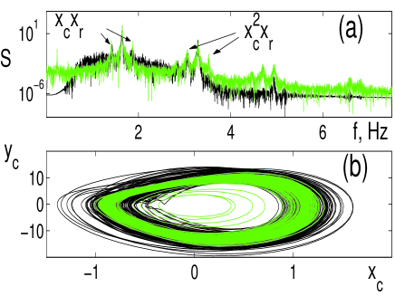
Figure 2: (a) Power spectra of cardiac oscillations obtained from measured data (black line) and from the synthesized model signal (green line). Arrows summarize combinational frequencies recovered in our analysis, corresponding to the nonlinear cardio-respiratory interaction. (b) Limit cycles of the cardiac oscillations $(x_{c}(n),y_{c}(n)$ obtained from measured data (black line) and the synthesized signal (green line).

The parameters of the model (6) can now be inferred directly from the measured time series of blood pressure, yielding the values shown in the first row of Table 1. The spectra of the inferred, $x_{r}(t)$, and the measured, $s_{r}(t)$, cardiac oscillations are compared in Fig. 2. Similar results are obtained for the respiratory oscillations. In particular, the parameters of the nonlinear coupling and of the noise intensity of the cardiac oscillations are $\beta_{20}=2.2,\beta_{21}=0.27$, $\beta_{22}=-8.67$, and $D_{22}=8.13$ ; here we use a double-indexing scheme for the coefficients of the linear expansion (Inference of a nonlinear stochastic model of the cardiorespiratory interaction), the scheme being evident from the caption in Table 1. It is clear that there is a close resemblance between the peaks at the basic and combinational frequencies, $nf_{c}+mf_{r}$, in the power-spectra. A similarly close resemblance is found for respiratory oscillations, $s_{r}(t)$ and $x_{r}(t)$, respectively (not shown).

The frequency content can be reproduced from a univariate signal $s(t)$ because for $f_{r}\ll f_{c}$ it can be written in the form: $s(t)\approx s_{r}(t)+A_{c}(t)\cos(f_{c}t+\theta_{c}(t))+\ldots$, here $A_{c}(t),\theta_{c}(t)$ are slow amplitude and phase and the omitted terms oscillate at multiples of $f_{c}$. Fast-oscillating terms in this expansion correspond to a cardiac signal $s_{c}(t)$ and this ensures the validity of the signal decomposition $s(t)=s_{r}(t)+s_{c}(t)$, with components corresponding to weakly coupled nonlinear oscillators.

$\alpha_{20}$	$\beta_{20}$	$\alpha_{21}$	$\beta_{21}$	$\alpha_{22}$	$\beta_{22}$	$D_{11}$	$D_{22}$
0.12	2.20	0.048	0.27	-0.066	-8.67	0.18	8.13
0.12	2.41	0.048	0.28	-0.070	-8.61	0.18	8.14
2.9%	9.3%	1.8%	5.6%	5.2%	0.7%	0.2%	0.2%

Table 1: Coefficients corresponding to the last three base functions in (Inference of a nonlinear stochastic model of the cardiorespiratory interaction), $\{x_{r}x_{c},x_{r}^{2}x_{c},x_{r}x_{c}^{2}\}$, with $\{\alpha_{i}\}$ corresponding to the respiration coupling to cardiac rhythm and $\{\beta_{i}\}$ to the cardiac oscillation coupling to respiration. The top row gives coefficients inferred from measured data. The middle row represents coefficients inferred from synthesized data, obtained as an average of 100 non-overlapped 1600 s blocks. Each block includes 160000 points with a sampling time 0.01 sec. The estimation error is shown in the bottom line.

To validate these results we consider a synthesized signal $x(t)=x_{r}(t)+x_{c}(t)$ where $x_{r}(t)$, $x_{c}(t)$ are obtained using numerical simulations of the model (3) with the parameters taken from the inference. We now repeat the full inference procedure to estimate nonlinear coupling parameters in (3) by using the synthesized univariate signal $x(t)$ as a time-series data input $s(t)$. This gives us the following estimates for the parameters of cardiac oscillations $\beta_{20}=6.32,\beta_{21}=0.49$, $\beta_{22}=6.03$, and $D_{22}=3.44$, which differ from the values in the first row of Table 1, but provides a correct estimation of the order of magnitude of the absolute values of the measured parameters. The main source of error here is the fact that we have to reconstruct the state of multidimensional system using the univariate signal.

If the state of the system was known the accuracy of inference could be arbitrary high Smelyanskiy:submitted . To illustrate this point we use the synthesized time-series $\{x_{r}(t),x_{c}(t),y_{r}(t),y_{c}(t)\}$ as bivariate data for two coupled oscillators to infer parameters of the model (3). The results are summarized in the second row of Table 1. It can be seen that the values of the parameters can be estimated with relative error of less than 10%. In particular, the relative error of estimation of the noise intensity is now below 4%. The accuracy of the estimation can be further improved by increasing the total time of observation of the system dynamics. The decomposition problem could of course be eliminated by using bivariate cardiovascular data, which are now commonly available.

The relative magnitudes of the parameters obtained, $|\beta_{i}|>|\alpha_{i}|$, indicate that respiration influences cardiac activity more strongly than vice versa, consistent with the results of methods specifically developed for detecting the coupling directionality of interacting oscillators Rosenblum:02Palus:03a , and with direct physiological observations. Furthermore, the presence of non-zero quadratic terms is consistent with recent results obtained by time-phase bispectral analysis Jamsek:03Jamsek:04 . The frequency and amplitude variability of the main oscillatory components Stefanovska:99a is implicitly captured within the coupling terms and noise. We find that the present model class is able to reproduce, not only the coupling directionality, but also to a large extent the 1:7 and 1:8 cardio-respiratory synchronization properties of the measured data, as will be discussed in detail elsewhere.

We would like to mention that reported method is only a first step in the direction of developing path-integral based approach to the dynamical inference of stochastic nonlinear models. It was verified on a number of model systems and has demonstrated stable and reliable inference of a broad class of models with high accuracy (see e.g. Smelyanskiy:submitted ). However, the method in its present form has a number of limitations. For example, to include frequencies lower then the frequency of respiration as well as to account for feedback mechanism of control from the nervous system will require for an extension of the model class used in the paper. In particular, it will require to include new degrees of freedom, time-delay functions and non-polynomial basis functions, possibly a non-white noise and non-parametric model inference. However, the technique can be readily extended to encompass mentioned above situations.

In summary, we have solved a long-standing problem in physiology: inference of a nonlinear model of cardio-respiratory interactions in the presence of fluctuations. Our technique estimates simultaneously the strength and directionality of coupling, and the noise intensity in the cardio-respiratory interaction, directly from measured time series. It can in principle also be applied to any physiological signal. Our solution is facilitated by an analytic derivation of the likelihood function that optimally compensates noise-induced errors in continuous dynamical systems. It has enabled us to effect the first application of nonlinear stochastic inference to identify a dynamical model from real data.

This work was supported by NASA CICT IS IDU project (USA), by the Leverhulme Trust and by EPSRC (UK), by the MŠZŠ (Slovenia), and by INTAS.

References

- (1) A. J. Camm et al., Circulation 93, 1043 (1996).
- (2) A. T. Winfree, The Geometry of Biological Time (Springer-Verlag, New York, 1980). L. Glass and M. C. Mackey, From Clocks to Chaos: The Rhythms of Life (Princeton University Press, Princeton, 1988).
- (3) D. L. Eckberg, J Physiol. 548, 339 (2003).
- (4) M. B. Visscher, A. Rupp, and F. H. Schott, Am. J. Physiol. 70, 586 (1924).
- (5) R. W. deBoer, J. M. Karemaker, and J. Strackee, Am. J. Physiol. 253, H680 (1987).
- (6) J. P. Saul, D. T. Kaplan, and R. I. Kitney, Computers in Cardiology (IEEE Comput. Soc. Press, Washington, 1988), pp. 299–302.
- (7) K. H. Chon, T. J. Mullen, and R. J. Cohen, IEEE Trans. Biomed. Eng. 43, 530 (1996). K. Suder, F. R. Drepper, M. Schiek, and H. H. Abel, Am. J. Physiol.: Heart. Circ. Physiol. 275, H1092 (1998).
- (8) A. Stefanovska and M. Bračič, Contemporary Physics 40, 31 (1999).
- (9) E. J. Kostelich, Physica D 58, 138 (1992). P. E. McSharry and L. A. Smith, Phys. Rev. Lett. 83, 4285 (1999).
- (10) M. Clynes, J. Appl. Physiol. 15, 863 (1960). G. Baselli, S. Cerutti, A. Malliani, and M. Pagani, IEEE Trans. Biomed. Eng. 35, 1033 (1988). B. J. TenVoorde et al., in Computer Analysis of Cardiovascular Signals, edited by M. Di Renzo et al (IOS Press, Amsterdam, 1995). H. Seidel and H. Herzel, in Modeling the Dynamics of Biological Systems, edited by E. Mosekilde and O. G. Mouritsen (Springer, Berlin, 1996), pp. 205–229. S. Cavalcanti and E. Belardinelli, IEEE Trans. Biomed. Eng. 43, 982 (1996). K. Kotani et al., Phys. Rev. E 65, 051923 (2002).
- (11) R. D. Berger, J. P. Saul, and R. J. Cohen, Am. J. Physiol.: Heart. Circ. Physiol. 256, H142 (1989). J. A. Taylor et al., Am. J. Physiol.: Heart. Circ. Physiol. 280, H2804 (2001). R. Mukkamala and R. J. Cohen, Am. J. Physiol.: Heart Circ. Physiol. 281, H2714 (2001). S. Lu, K. H. Ju, and K. H. Chon, IEEE Trans. Biomed. Engin. 48, 1116 (2001).
- (12) J. Jamšek, A. Stefanovska, P. V. E. McClintock, and I. A. Khovanov, Phys. Rev. E 68, 016201 (2003). J. Jamšek, A. Stefanovska, and P. V. E. McClintock, Phys. Med. Biol. 49, 4407 (2004).
- (13) C. Schäfer, M. G. Rosenblum, J. Kurths, and H. H. Abel, Nature 392, 239 (1998). N. B. Janson, A. G. Balanov, V. S. Anishchenko, and P. V. E. McClintock, Phys. Rev. Lett. 86, 1749 (2001).
- (14) M. G. Rosenblum et al., Phys. Rev. E. 65, 041909 (2002). M. Paluš and A. Stefanovska, Phys. Rev. E 67, 055201(R) (2003).
- (15) K. Visscher, M. J. Schnitzer, and S. M. Block, Nature 400, 184 (1999).
- (16) J. Christensen-Dalsgaard, Rev. Mod. Phys. 74, 1073 (2002).
- (17) A. Stefanovska and P. Krošelj, Open Syst. and Inf. Dyn. 4, 457 (1997). J. A. Taylor, D. L. Carr, C. W. Myers, and D. L. Eckberg , Circulation 98, 547 (1998). A. Stefanovska, D. G. Luchinsky, and P. V. E. McClintock, Physiol. Meas. 22, 551 (2001).
- (18) Alternative approaches could include e.g. empirical mode decomposition, Karhunen-Levé decomposition, or independent component analysis.
- (19) A. Stefanovska, M. Bračič Lotrič, S. Strle, and H. Haken, Physiol. Meas. 22, 535 (2001).
- (20) V. N. Smelyanskiy at el, cond-mat/0409282 (2004).
- (21) R. Graham, Z. Phys. B 26, 281 (1977).