Competitive Advantage for Multiple-Memory Strategies
in an Artificial Market

Abstract

We consider a simple binary market model containing $N$ competitive agents. The novel feature of our model is that it incorporates the tendency shown by traders to look for patterns in past price movements over multiple time scales, i.e. multiple memory-lengths. In the regime where these memory-lengths are all small, the average winnings per agent exceed those obtained for either (1) a pure population where all agents have equal memory-length, or (2) a mixed population comprising sub-populations of equal-memory agents with each sub-population having a different memory-length. Agents who consistently play strategies of a given memory-length, are found to win more on average – switching between strategies with different memory lengths incurs an effective penalty, while switching between strategies of equal memory does not. Agents employing short-memory strategies can outperform agents using long-memory strategies, even in the regime where an equal-memory system would have favored the use of long-memory strategies. Using the many-body ‘Crowd-Anticrowd’ theory, we obtain analytic expressions which are in good agreement with the observed numerical results. In the context of financial markets, our results suggest that multiple-memory agents have a better chance of identifying price patterns of unknown length and hence will typically have higher winnings.

1 INTRODUCTION

Complex systems are thought to be ubiquitous in the physical, biological and economic world. Research across these disciplines has focused increasingly on complex adaptive systems and their dynamical behavior. A noted feature of complex adaptive systems is that they can give rise to large macroscopic changes or ‘extreme events’ that appear spontaneously, have long-lasting consequences and yet seem to be very difficult to predict. Recent research [1, 2, 3] indicates, however, that predictability may be possible in certain instances. The models employed in such studies have typically involved individual, self-interested agents competing for a limited resource [1, 2, 3]. Research on these limited-resource agent games has so far been limited to ‘pure’ populations [4, 5, 6, 7, 8, 9] where all agents have the same memory-length m, and ‘alloy’ populations where the population of agents consists of sub-populations of equal $m$ but where $m$ varies from sub-population to sub-population [10].

In this paper we examine the effects of multiple-memory strategies in a multi-agent population. In particular, we consider the situation where the strategy set of an individual agent contains strategies with different memory-lengths m. When the memory-lengths are sufficiently small, these multiple-memory agents outperform both a pure population of equal-memory agents, and an alloy population comprising sub-populations of equal-memory agents. Agents who consistently play strategies of a given memory length, are found to win more on average – switching between strategies with different memory lengths incurs an effective penalty, while switching between strategies of equal memory does not. We find that agents choosing to use short-memory strategies can outperform agents using long-memory strategies – remarkably, this is true even in the regime where an equal-memory system would have favored the use of long-memory strategies. Using the many-body ‘Crowd-Anticrowd’ theory [5] we obtain analytic expressions which are in good agreement with the observed numerical results. In the context of financial markets, our results suggest that multiple-memory agents have a better chance of identifying price patterns of unknown length and hence will typically have higher winnings. In other words, agents who are capable of looking for patterns in past outcomes over several timescales, will do better on average.

Our artificial market takes the form of a binary agent resource (B-A-R) game [5, 11] of which a special limiting case is the so-called Minority Game[4, 5]. The market consists of an odd number of agents (e.g. traders) $N$, of which no more than $L<N$ agents can be rewarded at each time step. At each time step $t$ each agent $i$ makes a decision ${a_{i}}(t)$ to buy (${a_{i}}(t)=1)$ or sell (${a_{i}}(t)=0$). If $\sum_{i=1}^{N}{a_{i}}(t)>L$ then at time step $t$ all agents who chose ‘0’ are rewarded, otherwise all agents who chose ‘1’ are rewarded. As a specific example in this paper, we take N to be odd, and set $L=(N-1)/2$ which results in more losers than winners at each time step as in the Minority Game. Elsewhere we give the corresponding results for general $L$. This artificial market provides a simple paradigm for the dynamics underlying financial markets: more sellers than buyers implies lower prices, thus it can be better for a trader to be in the smaller group of buyers. The ‘output’ of the market is a single binary digit, 0 or 1 (0 if $\sum_{i=1}^{N}{a_{i}}(t)>L$, otherwise 1). This is the only information that is available to the agents. Agents with strategies of memory size m therefore have access to the last m binary output digits $\mu_{m}$ when making their decisions. Agents who possess multiple strategies of different memory lengths will therefore use different information when deciding which action to take at the next time step. Using information from different history lengths can be interpreted as somewhat analogous to the techniques of ‘chartists’ for making forecasts. Indeed, it is well known that in practice a financial trader’s computer screen displays past price movements over several different timescales (e.g. hours, days, weeks).

We consider our N-agent population to possess strategies drawn from a strategy pool which corresponds to memory lengths $m_{1}$ and $m_{2}$. At the beginning of the game the agents are randomly assigned $s$ strategies, of which $s_{1}$ strategies are of memory length $m_{1}$ and $s_{2}$ strategies are of memory length $m_{2}$ with repetitions allowed. The total number of strategies for each agent is the same, i.e. $s=s_{1}+s_{2}$. A strategy is a mapping from the length $m$ recent-history bit-string onto a binary decision $\mu_{m}\rightarrow\{0,1\}$. Consider $m=3$. There are $2^{2^{m}}=256$ possible strategies, each of which can be represented by a string of 8 bits (0 or 1) corresponding to the decisions based on the $2^{m}=8$ possible histories $\mu_{m}$ (e.g. 000, 001, etc). For example, the $m=3$ strategy $01101000$ represents the mapping $\{000\rightarrow 0,001\rightarrow 1,010\rightarrow 1,011\rightarrow 0,100\rightarrow 1,101\rightarrow 0,110\rightarrow 0,111\rightarrow 0\}$.

On every time step, the agent is awarded one point if the strategy he chose to use does actually predict the correct global output. In addition, he compares the prediction of all of his strategies to the correct global output. Each strategy that predicted the correct global output receives one ‘virtual’ point, and each strategy that predicted the wrong global output loses one ‘virtual’ point. Thus at each time step, each agent has a running tally of how successful each of his s strategies has been. On each time step an agent picks the most successful strategy (with the highest ‘virtual’ point score) as his decision. If two or more strategies have the same ‘virtual’ point score the agent randomly chooses between the tied strategies with equal probability. The success of any particular strategy generally fluctuates. As agents begin to use similar strategies, those strategies become less profitable, causing the agents to switch to a different strategy. Therefore there is no best strategy for all times.

The full strategy space (FSS) forms a $2^{m}$-dimensional hypercube for memory length $m$ with a unique strategy at each of the $2^{2^{m}}$ verticies [4, 5]. In general, the game’s dynamics can be reproduced by considering a reduced strategy space (RSS) containing only $2\times 2^{m}$ strategies, where each strategy is either anti-correlated or uncorrelated to the rest of the strategies in the RSS [12]. This reduction of the FSS to RSS has the effect of retaining the strong correlations in the system, which in turn tend to drive the dynamics, while removing the weak ones which just tend to create minor fluctuations. If the total number of strategies in play is greater than the size of the reduced strategy space (i.e. $N\times s\gg 2\times 2^{m}$) many agents may hold the highest-scoring strategy at any given time step. This will cause a large number of agents to play the same strategy, which will lead to a large disparity between the number of agents who chose winning and losing market actions (i.e. $\sum_{i=1}^{N}{a_{i}}(t)\gg L$ or $\sum_{i=1}^{N}{a_{i}}(t)\ll L$) and a relatively low number of total points awarded [4, 5] since the total number of points awarded at each time step is given by $(N-{\rm abs}[\sum_{i=1}^{N}{a_{i}}(t)-L-0.5]-0.5)/2$. Such crowd effects are a strategy-space phenomenon and have been shown to quantitatively explain the fluctuations in the number of winning agents per turn for the pure population as a function of $m$ and $s$ [5]. Furthermore, the most number of points that can be awarded on a given time step is $(N-1)/2$ and hence the average winnings (total points awarded) per agent per turn, $W$, is always less than or equal to $(N-1)/2N$, hence $W<0.5$. When $N\times s\gg 2\times 2^{m}$, $W$ is substantially less than 0.5 due to the crowd effects mentioned above. Note that an external (i.e. non-participating) gambler using a ‘coin toss’ to predict the winning room, would have a $50\%$ success rate since he would not suffer from this intrinsic crowding in strategy space.

The dynamics of the artificial market also depend on the trajectory which the game follows in the history space $\{\mu\}$. The history space forms an m-dimensional hypercube whose $2^{m}$ vertices correspond to all possible history bit-strings of length $m$. In the crowded regime (i.e. $N\times s\gg 2\times 2^{m}$) there is information left in the history time series that is inaccessible by a pure population of agents with memory $m$, since this information is contained within bit-strings of length greater than $m$. When the total number of strategies held by the agents is only a small subset of the RSS, agents are not able to fully extract the information contained in bit-strings of any length (including $\leq m$) [5, 10]. Cavagna claimed [13] that it is irrelevant whether one uses the real history or random history as an input to the agents in the Minority Game [13]. However Johnson et al. subsequently showed [10] that in an alloy population of agents, for example, the trajectories through history space do indeed become important. In particular, higher $m$ agents have the opportunity to exploit specific correlations in the real-history time series left by the lower $m$ agents.

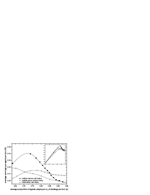
Figure 1: Average winnings per agent per turn, $W$, for multiple-memory populations and a mixed-ability population with $N=101$, $m_{1}=3$ and $m_{2}=6$, as obtained numerically. Each agent has $s=16$ strategies. Each data-point corresponds to an average over 25 simulations. The connecting curves are a guide to the eye. The inset shows $W$ over the full range of $x$, where $x$ is the average proportion of agents playing an $m_{2}=6$ strategy per turn. See the text for an explanation of ‘real history’ and ‘random history’.

2 RESULTS

Figure 1 shows the average winnings per agent per turn, $W$, for two multiple-memory populations (circles) and a mixed-ability population (crosses). All three populations correspond to $N=101$ agents and $s=16$ strategies per agent. In the mixed-memory population, $N_{m_{1}}$ agents hold strategies of memory-length $m_{1}=3$, while $N-N_{m_{1}}$ agents hold strategies of memory-length $m_{2}=6$. In the multiple-memory populations, each agent holds $s_{1}$ strategies of memory-length $m_{1}=3$ and $s_{2}$ strategies of memory-length $m_{2}=6$. The curves are plotted against $x$, the average proportion of agents playing an $m_{2}$ strategy on each turn. For the mixed-ability population, the average proportion of agents playing an $m_{2}$ strategy is simply $(N-N_{m_{1}})/N$. For the multiple-memory populations, we determined numerically the average number of agents playing an $m_{2}$ strategy at each turn, and divided that number by $N$. Each data point represents an average over 25 runs. The results for the multiple-memory population are averaged over both $W$ and $x$, since in the multiple-memory population $s_{1}$ and $s_{2}$ are exogenously determined whereas $x$ is endogenous (see Figure 2). For clarity we have not shown the error bars for each data point – however the range of values in both $W$ and $x$ is sufficiently small that our results, discussions and conclusions are not affected by numerical artifacts. Agents are supplied with the $m_{1}$ (and/or $m_{2}$) most recent winning actions of the artificial market in the ‘real-history’ results (solid circles for the multiple-memory population). For the ‘random-history’ results (open cirles for the multiple-memory population) agents are given a random $m_{1}$ (and/or $m_{2}$) length bit-string every time step instead of the actual bit-string of winning market actions. (For random-history results for a mixed-ability population, see Johnson et. al.[10]). The ‘real-history’ multiple-memory population exhibits a maximum in $W$ at a finite value of $x\sim.72$. We find that as $s$ increases the value of $x$ that maximizes $W$ asymptotically approaches $\sim.76$ (we have investigated cases up to $s=100$). The total number of points awarded per turn can therefore exceed either a pure $m_{1}=3$ or pure $m_{2}=6$ population of agents. The ‘random-history’ multiple-memory population also exhibits a maximum at a finite value of $x$. However, the magnitude of the difference between $W_{\rm{max}}$ and $W$ when $x=1$ (i.e. a pure $m_{2}$=6 population) is only $\sim 0.007$, which is within the standard deviation of the values of $W$. Hence the ‘random-history’ multiple-memory population does not significantly outperform a pure $m_{2}=6$ population. Therefore, history has a significant effect on the ability of a multiple-memory population to outperform a pure population. In other words, a multiple-memory population can collectively profit from the real patterns which arise in past outcomes – most importantly, this added benefit of multiple-memory does not arise simply from a reduction in crowding in the strategy space. For all values of $x$, the average winnings per agent per turn of the ‘real-history’ multiple-memory population, is greater than or equal to the average winnings per agent per turn for the mixed-ability population. This result is not duplicated if the multiple-memory population is presented with a random history string. Multiple-memory agents that are presented with the real history of winning actions from the artificial market can therefore outperform both pure populations of agents holding strategies of memory length $m_{1}$ or $m_{2}$ and simultaneously outperform a mixed-ability population consisting of sub-populations of agents with $m_{1}$ or $m_{2}$ strategies.

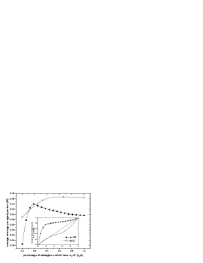
Figure 2: Average winnings per agent per turn, $W$, for multiple-memory populations with $s=16$ and $s=3$. Other parameters are as in Fig. 1. The inset shows the average proportion $x$ of agents playing an $m_{2}$ strategy for the same two populations. The dotted line in the inset represents the line $x=s_{2}/s$.

Figure 2 shows the average winnings per agent per turn $W$ for two multiple-memory populations. Both populations are given the real history bit-string. One population has $s=16$ (solid circles) as above, while the other population has $s=3$ (triangles). All other relevant parameters are the same as in Fig. 1, however we now plot $W$ against the exogenously controlled proportion of $m_{2}$ strategies (i.e. $s_{2}/s$). Both $s=16$ and $s=3$ multiple-memory populations exhibit a maximum in $W$ at finite $s_{2}/s$, again showing that the multiple-memory populations can outperform pure populations. As $s$ increases, the value of $s_{2}/s$ which maximizes $W$ tends towards 0. However, for $7\leq s\leq 100$ we find that $W$ is always maximized when $s_{2}=3$. We find a similar result for multiple-memory populations with $m_{1}=1$ and $m_{2}=2$ – in this case, $W$ is always maximized when $s_{2}=1$. In the inset to Fig. 2, we plot the average proportion of agents who play an $m_{2}=6$ strategy per turn (i.e. $x$) versus $s_{2}/s$. The circles and triangles represent the same multiple-memory populations as described above, and the straight dashed line corresponds to $x=s_{2}/s$. Neglecting the endpoints, $x$ for the $s=16$ multiple-memory population always lies above the dashed line. Agents are therefore playing their $m_{2}$ strategies at a higher rate than if they were choosing a strategy at random each turn. This result is not too surprising, since we expect the $m_{2}$ strategies to outperform the $m_{1}$ strategies – after all, a pure $m_{2}$ population will have a higher $W$ than the corresponding pure $m_{1}$ population. However when $s=3$ (or $s=2$), and neglecting the endpoints, $x$ lies below the dashed line. Therefore in a multiple-memory population with low $s$, agents play $m_{1}$ strategies more frequently than the proportion of $m_{1}$ strategies that they hold. This result is remarkable since a pure $m_{2}=6$, $s=3$ population is known to outperform a pure $m_{1}=3$, $s=3$ populations. The agents who play $m_{1}$ strategies more than half the time (i.e. agents with $x<0.5$) have higher average winnings per turn than agents who play $m_{2}$ strategies more than half the time. This is illustrated in Fig. 3.

Figure 3: Average winnings per turn, $W$, for multiple memory populations with $s=3$ (top) and $s=16$ (bottom). Each data-point represents a single agent. Other parameters are as in Fig. 2.

In the top half of Fig. 3, we plot the average winnings per turn for 2525 agents (25 runs, $N=101$ each run) versus the proportion of turns in which an agent played an $m_{2}$ strategy. Each agent has $s=3$ strategies, with $s_{1}=1$, $m_{1}=3$, $s_{2}=2$ and $m_{2}=6$. Agents who consistently play an $m_{1}$ or $m_{2}$ strategy have, on average, higher average winnings than agents who play a combination of $m_{1}$ and $m_{2}$ strategies. In a pure population, agents who play a combination of their strategies also tend to incur an effective penalty. However, we find that the penalty for switching between strategies of different memory lengths is greater and more certain, i.e. $W$ is on average lower and the spread of $W$ values is also smaller. In the bottom half of Fig. 3, we plot the average winnings per turn for 2525 agents versus the proportion of turns in which an agent played an $m_{2}$ strategy. All parameters are the same as for the top figure, except now we have set $s=16$, with $s_{1}=13$ and $s_{2}=3$. With increasing $s$ it is clear that there is an effective penalty for playing an $m_{1}$ strategy. Agents who consistently play $m_{2}$ strategies achieve winning percentages higher than 0.5, or that which could be achieved by an external player using a random coin toss to predict the winning market decision. The average winnings per turn for agents who always play $m_{2}$ strategies is $\sim 0.5$.

Figure 4 shows the standard deviation in the excess demand for a multiple-memory population (solid circles) as a function of the percentage of strategies which have $m_{2}=6$. The parameters for the populations are the same as for the $s=16$ multiple-memory population discussed above. The excess demand for our artificial market is the difference between the number of agents who choose to ‘buy’ and ‘sell’ at each time step. The closer the excess demand is to zero, the higher the number of total points which are awarded each turn. The standard deviation in the excess demand can serve as a proxy for the wastage in the system. The more the standard deviation of excess demand fluctuates each turn, the smaller the total number of points that can be awarded to agents. The population exhibits a minimum in the standard deviation of excess demand at finite $s_{2}/s$, and at exactly the same value of $s_{2}/s$ which maximizes the average winnings per agent per turn (see Fig. 2). The empty circles represent the standard deviation of the excess demand as predicted by the Crowd-Anticrowd theory, which is discussed in the following section. In the inset we plot the standard deviation in excess demand for an $s=8$ multiple-memory population, with all other parameters being the same as in the main figure.

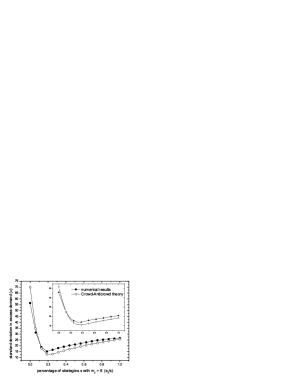
Figure 4: Standard deviation in the excess demand $\sigma$ for multiple memory populations with $s=16$ and $s=8$ (inset) obtained numerically (solid circles) and as predicted by the Crowd-Anticrowd theory (empty circles). Other parameters are as in Fig. 1. See text for an explanation of excess demand and Crowd-Anticrowd theory.

3 DISCUSSION

Our numerical results demonstrate that populations of agents with multiple-memory strategies can outperform both pure populations of agents and mixed-ability populations. This comparative advantage can be explained through the framework of the Crowd-Anticrowd theory. As a first approximation, we treat the two groups of agents playing $m_{1}$ and $m_{2}$ strategies on a given turn as independent, as per the mixed-ability population. Thus we examine the Crowd-Anticrowd theory as applied to a mixed-ability population. Considering the action of different sub-populations of agents as uncorrelated, the variance in the excess demand for a mixed-ability population goes as $\sigma^{2}=\sigma_{1}^{2}+\sigma_{2}^{2}$. Here $\sigma_{1}^{2}$ ($\sigma_{2}^{2}$) is the variance due to the population of $m_{1}$ ($m_{2}$) agents, where $\sigma_{1}^{2}=C^{2}(m_{1},s_{1})(1-x)^{2}N^{2}$ and $\sigma_{2}^{2}=C^{2}(m_{2},s_{2})(1-x)^{2}N^{2}$. The pre-factor $C^{2}(m_{i},s_{i})$ is a constant of proportionality, and $x$ is the proportion of agents playing an $m_{2}$ strategy. The standard deviation in excess demand can thus be calculated as:

$$\sigma=N[C^{2}(m_{1},s_{1})(1-x)^{2}+C^{2}(m_{2},s_{2})x^{2}]^{1/2}.$$ (1)

For mixed-ability populations $x$ is exogenously determined. However in the multiple-memory population, $x$ is determined by the relative success of strategies with different memory-lengths. Therefore we must develop an expression for how agents choose to segregate themselves between playing the $m_{1}$ and $m_{2}$ strategies.

In order to understand how agents will choose between $m_{1}$ and $m_{2}$ strategies, we must consider how the strategy spaces are related. Every strategy in the $m_{1}$ space maps uniquely to a strategy in the $m_{2}$ space. For example, take $m_{1}=3$, $m_{2}=6$ and the $m_{1}$ strategy $01101000$. This strategy is equivalent to the $m_{2}$ strategy $0110100001101000011010000110100001101000011010000110100001101000$. In the Crowd-Anticrowd theory, we assume that on each time step the ranking of strategies according to success rate and popularity are equivalent. As there is a one-to-one mapping from $m_{1}$ strategy space to $m_{2}$ strategy space, we will assume that the relative rankings are also preserved in the mapping from $m_{1}$ space to $m_{2}$ space, i.e. if strategy $A_{m_{1}}$ is more popular than $B_{m_{1}}$, then we assume that $A_{m_{2}}$ is more popular than $B_{m_{2}}$). Next we assume that an $m_{2}$ strategy will, with probability $p$, have a higher ranking than an agent’s best $m_{1}$ strategy. Therefore, the agent will play an $m_{2}$ strategy with probability

$$x=1-(1-p)^{(s-s_{1})},$$ (2)

where $s$ is the total number of strategies an agent possesses, and $s_{1}$ is the number of $m_{1}$ strategies that the agent possesses. In order to determine the value for $p$, we must first calculate the expected value of the ranking $k$ for the agent’s highest-ranked $m_{1}$ strategy as a function of $s_{1}$ and $m_{1}$:

$$E[k_{\rm{max}}|s_{1}]=2P_{1}(1-{s_{1}\over s_{1}+1})$$ (3)

where $P_{1}=2^{m_{1}}$. If we analyze the strategies in terms of the RSS, the $m_{1}$ strategies ranked from 1 to $P_{1}$ must map to $m_{2}$ strategies in the ranked set ${1..P_{2}}$. This is a consequence of the fact that every strategy in the RSS is either anticorrelated or uncorrelated to every other strategy in the RSS. If both strategy spaces are in the crowded regime (i.e. $Ns_{1}\gg 2P_{1}$ and $Ns_{2}\gg 2P_{2}$) and the $m_{2}$ strategy space is significantly larger than the $m_{1}$ strategy space (i.e. $P_{2}/P_{1}\gg 1$) then the mapping of the ranking of $m_{1}$ strategies will fall into the middle range of strategy-rankings of $m_{2}$ space. (This assumption should hold if $Ns_{1}/2P_{1}\gg Ns_{2}/2P_{2}$). For example, since ordering is preserved, the strategy with $k=1$ in the $m_{1}$ RSS maps to $k=P_{2}-P_{1}+1$ in $m_{2}$ RSS. Thus the probability that an $m_{2}$ strategy is better than the current most popular $m_{1}$ strategy, is $1-[(P_{2}-P_{1}+1)/2P_{2}]=(P_{2}+P_{1}-1)/2P_{2}$. More generally, the best $m_{1}$ strategy that an agent possesses is the $k_{\rm{max}}$th most popular one, given by Equation 3. The general expression for $p$ then becomes

$$p={P_{2}+P_{1}(1-s_{1}/(s_{1}+1))-1\over 2P_{2}}.$$ (4)

Our theoretical predictions for the standard deviation of the excess demand are plotted in Fig. 4. The agreement with the numerical results is very good. We also note that this agreement actually improves with increasing $s$, a feature that would be very hard to reproduce in comparable spin-glass based theories .

One of the limitations of our theory as outlined so far, is the assumption that the actions of the agents playing an $m_{1}$ strategy is uncorrelated to the actions of agents playing an $m_{2}$ strategy. As discussed above, the $m_{2}$ RSS covers the $m_{1}$ RSS – therefore we need to modify Eq. 1 by adding a covariance term. The specific details of the covariance term will be presented elsewhere. For now, we just comment on the fact since there is likely to be additional crowding that is unaccounted for, this covariance should be positive and will decrease with increasing $x$ and $m_{2}$. We also expect that our expression for $x$ will be an overestimation, since we have assumed that the most popular $m_{1}$ strategy is ranked as low as it possibly can be in the $m_{2}$ RSS. We believe that these two factors explain why our theoretical predictions for the standard deviation in the excess demand slightly underestimate the numerical results for the multiple-memory populations. We can therefore conclude that multiple-memory populations gain their comparative advantage by behaving as mixed-ability populations with fewer strategies. Additional strategies in the multiple-memory populations will cause the standard deviation in the excess demand to approach the random limit. However, the rate is far slower than in the case of either pure populations or mixed-ability populations.

In game realizations where both the $m_{1}$ RSS and $m_{2}$ RSS are not crowded (e.g. as in the $s=3$ multiple-memory populations in Figs. 2 and 3) our simple theory for $x$ does not hold. In cases where one of the RSS is not crowded, the highest ranked $m_{1}$ strategy can map to a higher-ranked $m_{2}$ strategy than we had assumed above. This causes the value for $p$ to be reduced, and could in certain cases cause $x$ to fall below $s_{2}/s$ as in the $s=3$ case above. We suspect that this effect is related to the information in the history string. If the $m_{1}$ agents can fully access the information in the $m_{1}$ length bit-string, but there are insufficient $m_{2}$ strategies to access the additional information in the $m_{2}$ length bit-strings, it may be more advantageous to play an $m_{1}$ strategy. This conjecture is reinforced by the importance of memory in the multiple-memory populations, which we believe is related to the different time scales being tracked by the system. When neither of the RSS are crowded, we expect $x\sim s_{2}/s$. (This result has been confirmed in numerical simulations with $m_{1}=10$ and $m_{2}=13$).

In conclusion, we have studied the performance and dynamics of a population of multiple-memory agents competing in an artificial market. We have shown that multiple-memory agents possess a comparative advantage over both pure populations of agents and mixed-ability populations. We have presented a theory based on the Crowd-Anticrowd theory, which is in good agreement with these numerical results.

- [1] See M. Buchanan’s article in New Scientist, 26 February (2005), p. 32.
- [2] D.M.D. Smith and N.F. Johnson, preprint cond-mat/0409036; D. Lamper, S.D. Howison and N.F. Johnson, Phys. Rev. Lett. 88, 017902 (2002); N.F. Johnson, D. Lamper, P. Jefferies, M.L. Hart, S. Howison, Physica A 299, 222 (2001).
- [3] J. V. Andersen and D. Sornette, preprint cond-mat/0410762.
- [4] D. Challet, Y. C. Zhang, Physica A 246, 407 (1997); D. Challet, M. Marsili, and R. Zecchina, Phys. Rev. Lett. 84, 1824 (2000); R. Savit, R. Manuca, and R. Riolo, Phys. Rev. Lett. 82, 2203 (1999); N. F. Johnson, P. M. Hui, R. Jonson, and T. S. Lo, Phys. Rev. Lett. 82, 3360 (1999); S. Hod and E. Nakar, Phys. Rev. Lett. 88, 238702 (2002).
- [5] N.F. Johnson and P.M. Hui, preprint cond-mat/0306516; N.F. Johnson, S.C. Choe, S. Gourley, T. Jarrett, P.M. Hui, Advances in Solid State Physics, 44, 427-438 (Springer Verlag, Germany, 2004); M. Hart, P. Jefferies, N. F. Johnson, P. M. Hui, Physica A 298, 537 (2001); N.F.Johnson, P. Jefferies, P.M. Hui, Financial Market Complexity (Oxford University Press, Oxford, 2003).
- [6] A. Cavagna, J. P. Garrahan, I. Giardina, and D. Sherrington, Phys. Rev. Lett. 83, 4429 (1999); M. Hart, P. Jefferies, N. F. Johnson, P. M. Hui, Phys. Rev. E 63, 017102 (2000).
- [7] M. Anghel, Z. Toroczkai, K.E. Bassler, G. Korniss, Phys. Rev. Lett. 92, 058701 (2004); I. Caridi, H. Ceva, cond-mat/0401372; M. Sysi-Aho, A. Chakraborti, and K. Kaski, Physica A 322, 701 (2003); D. Challet, M. Marsili and G. Ottino, preprint cond-mat/0306445.
- [8] S. Gourley, S.C. Choe, N.F. Johnson and P.M. Hui, Europhys. Lett. 67, 867 (2004).
- [9] S.C. Choe, N.F. Johnson and P.M. Hui, Phys. Rev. E 70, 055101(R), (2004).
- [10] N.F. Johnson, P.M. Hui, D. Zheng, and M. Hart, J. Phys. A: Math. Gen. 32, L427 (1999).
- [11] W.B. Arthur, Science 284, 107 (1999); W. B. Arthur, Am. Econ. Assoc. Papers Proc. 84, 406 (1994); N. F. Johnson, S. Jarvis, R. Jonson, P. Cheung, Y. R. Kwong and P. M. Hui, Physica A 258, 230 (1998).
- [12] See for example, P. Jefferies, M.L. Hart and N.F. Johnson, Phys. Rev. E 65, 016105 (2002).
- [13] A. Cavagna, Phys. Rev. E 59, R3783 (1999).