Statistical Properties of Demand Fluctuation in the Financial Market

Abstract

We examine the out-of-equilibrium phase reported by Plerou et. al. in Nature, 421, 130 (2003) using the data of the New York stock market (NYSE) between the years 2001 –2002. We find that the observed two phase phenomenon is an artifact of the definition of the control parameter coupled with the nature of the probability distribution function of the share volume. We reproduce the two phase behavior by a simple simulation demonstrating the absence of any collective phenomenon. We further report some interesting statistical regularities of the demand fluctuation of the financial market.

Recently a report based on New York stock exchange (NYSE) data between period 1995-1996 ref. Stanley1 reported that the financial market has two phases, namely, the “equilibrium” phase, and the “out-of-equilibrium” phase. Ref. Stanley1 further reported a critical point which is the boundary between a $0$ and finite value of the order parameter for the observed phase transition.

In this paper we address the following questions in an effort to understand the observed two phase phenomenon:

1. What is the cause of the observed two phase behavior ?

2. Do large changes of price occur in out-of-equilibrium phase ?

Our study is based on the NYSE Trades and Quotes (TAQ) database for the period 2001–2002 which records every ask, bid, and transaction price.

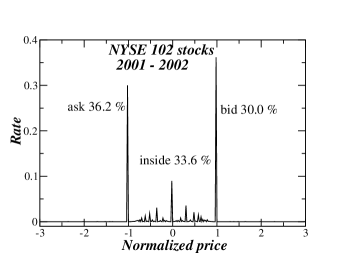
Figure 1: Percentage of transactions occurring at ask, bid and/or an intermediate price between ask and bid prices which are normalized to +1 and -1, respectively. We observe that nearly 1/3 of the transactions take place in each one of these three groups.

Figure 1 gives an estimate of the percentage of transactions during the period period 2001–2002 that was either at the ask price (scaled to be 1), at the bid price (scaled to be -1), or at an intermediate value between the ask and the bid prices.

Using the method of ref. Stanley1 we first identify a buyer initiated or a seller initiated transaction by a quantity $a$ which is defined as follows:

$$a=\left\{\begin{array}[]{l}\hskip 5.69046pt1\hskip 14.22636pt\mathrm{if}~{}~{}~{}p>(ask-bid)/2\\ \hskip 5.69046pt0\hskip 14.22636pt\mathrm{if}~{}~{}~{}p=(ask-bid)/2\\ -1\hskip 14.22636pt\mathrm{if}~{}~{}~{}p<(ask-bid)/2\\ \end{array}\right.$$ (1)

where $p$ is a transaction price. Usually a transaction is executed when a new quote hits the lowest ask price or the highest bid price.

As in ref. Stanley1 , we define the volume imbalance $\Omega$ and its standard deviation as

$$\Omega(t)=\sum\limits_{i=1}^{N(t)}{q_{i}a_{i}}$$ (2)

$$\Sigma(t)=<|q_{i}a_{i}-<q_{i}a_{i}>_{t}|>_{t}$$ (3)

where $q_{i}$ is the share volume of the $i$th transaction within the period $\Delta t$.

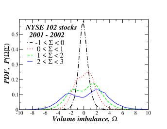
Figure 2: Probability density function $P(\Omega|\Sigma)$ for given $\Sigma$. We observe that P($\Omega|\Sigma$) for $\Sigma>0$. Reference Stanley1 interprets the two maximas of P($\Omega|\Sigma$) as the two phases of the financial market.

Fig. 2 displays the probability density function (PDF) $P(\Omega|\Sigma)$ of $\Omega$ for a given $\Sigma$. We observe a bi-modal PDF with two extrema when $\Sigma$ is larger than a critical value. This feature of $P(\Omega|\Sigma)$ is reported as an instance of two phase behavior in the financial market [Fig. 1 (a)of ref. Stanley1 ].

We next accumulate the $a$ between intervals $t$ and $t+\Delta t$ to estimate a quantity $\Phi=\sum\limits_{i=1}^{N(t)}{a_{i}}$ which measures the number imbalance between buyer and seller initiated trade within the time interval $\Delta t$.

The first moment $\sigma$ of $\Phi$ is defined as

$$\sigma(t)=<|a_{i}-<a_{i}>_{t}|>_{t}$$ (4)

where $<...>_{t}$ represents an average in the time interval $\Delta t$ .

We also define

$$q(t)=\frac{1}{N(t)}\sum_{i=1}^{N(t)}q_{i}$$ (5)

which measures the average volume of trade per transactions between $t$ and $t+\Delta t$.

We estimate $~{}\Omega(t),~{}\Sigma(t)$, and $q(t)$ averaged over 102 stocks which has the largest total volume among all NYSE stocks in 2002 with $\Delta t=15$ minutes. .

In phase transitions observed in physical systems, the control parameters are independent variables. But in ref. Stanley1 , the control parameter $\Sigma$ is the magnitude of fluctuation of the order parameter $\Omega$. When fluctuations are large, the underlying PDF of the random variable is wide, leading us to think that we might replicate $P(\Omega|\Sigma)$ by simulation.

First we evaluate the empirical correlations present in the database between different variables defined in eq. 1–5. Table 1 tabulates the estimated correlations.

Table 1: Correlations

	$|R|$	$N$	$q$	$\Sigma$	$\sigma$
$|R|$	1.00	0.10	0.20	0.11	0.11
$N$	-	1.00	0.03	0.01	0.50
$q$	-	-	1.00	0.69	0.14
$\Sigma$	-	-	-	1.00	0.08
$\sigma$	-	-	-	-	1.00

Next, for simulation, we consider $a$, $q$, and $N$ to be identically and independently distributed (i.i.d) from two possible PDFs given in Table 2 Stanley2 . We execute the simulation for eight ($2^{3}$) possible combinations of the set $a$, $q$ and $N$.

Table 2: Different combinations of $a$, $q$ and $N$ for simulation.

$a$	random 1,-1	Normal(0,1)
$q$	power law $q^{-1.5}$	Normal(10,3)
$N$	power law $N^{-3.4}$	Normal(10,3)

Since $a$, $q$, and $N$ are i.i.d, there are no autocorrelations like that in the TAQ time series, but even then, in we find $P(\Omega|\Sigma)$ to have a bi-modal distribution only when the PDF of the share volume is a power law (c.f. Fig 3). This observation can be explained as follows: First note that the PDF $P(q)$ of $q$ has the functional form of a power law, i.e., $P(q)\sim q^{-1.5}$. Next note that the $\Omega$ has a $q$ in its definition, thus the PDF $P(\Omega)$ of $\Omega$ also has the functional form of a power law. Occurrence of extreme positive and negative events are much more probable when $P(\Omega)$ has a fat tail. Since $\Sigma$ by definition is the standard deviation of the random variable $\Omega$, large values of $\Sigma$ occur when extreme events (both positive and negative) of $\Omega$ are sampled. Thus $P(\Omega|\Sigma)$ has two extrema resulting from large positive and negative sampling of the random variable $\Omega$ when we choose groups with large $\Sigma$ values [c.f. Fig. 3(a) and  3(c)].

Table 3 tabulates the estimated correlations between the pairs $q$, $\Sigma$, and $N$, $\Sigma$ for the case of TAQ database and simulation. We find correlation values for the TAQ database and simulation to be statistically similar when $q$ and $N$ are power law distributed, which further demonstrates that the observed two phase effect is not a signature of hidden collective phenomena within financial market. An explanation similar to the one above is reported in ref. Bouchaud .

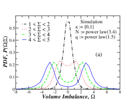
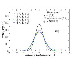
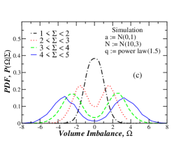
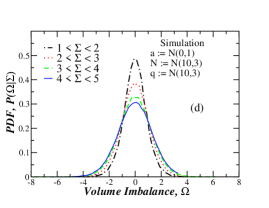
Figure 3: $P(\Omega|\Sigma)$ with $\Omega$ and $\Sigma$ generated from i.i.d., for four different combinations of $a,~{}q,~{}N$. We observe a bi-modal distribution of $P(\Omega|\Sigma)$ only when $P(q)$ has a power law functional form. Since $P(q)\sim q^{-1.5}$ and the definition of $\Omega$ has $q$ in its argument, $P(\Omega)$ also has the functional form of a power law. Thus for the power law distributed $P(\Omega)$ occurrence of extreme positive and negative events are much more probable than if $P(\Omega)$ did not have a fat tail. $\Sigma$ by definition is the standard deviation of the random variable $\Omega$. Large values of $\Sigma$ occurs when extreme events (both positive and negative) are sampled. Thus $P(\Omega|\Sigma)$ has two extremas resulting from a large positive and negative sampling of the random variable $\Omega$ when groups with large $\Sigma$ values are chosen [c.f. (a) and (c)].

Table 3: Correlations of pair $(q,\Sigma)$ and $(N,\Sigma)$.

Correlation	$(q,\Sigma)$	$(N,\Sigma)$
TAQ 2000-2001 database	0.69	0.01
Simulation with $q$, $N$
distributed as in Fig 3a	0.95	0.00
Simulation with $q$, $N$
distributed as in Fig 3b	0.08	0.03
Simulation with $q$, $N$
distributed as in Fig 3c	0.71	0.00
Simulation with $q$, $N$
distributed as in Fig 3d	0.19	0.11

To examine this in closest detail, we next estimate the PDF of $q$ and $N$ for a given $\Sigma$ from the TAQ database. Fig.4(a) show, that $q$ is large for large $\Sigma$. Fig.4(b) shows that $N$ is almost independent of $\Sigma$. By this, we can infer that the bi-modal PDF $P(\Omega|\Sigma)$ is caused by the transactions of large investors with large number of shares. The small decrease in $<N>$ as $\Sigma$ increases has a simple explanation, which was pointed out by our referee. In normal markets the specialist, whose role is to maintain a fair and orderly market, crosses the book via his clerk very regularly in an almost automated fashion. When fluctuations become large the specialist must take a close look at the electronic order book and at the order from the floor before he may decide which and at what price it is fair to cross the orders. This manual intervention takes time and is a plausible cause of the decrease in the number of trades.

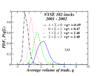
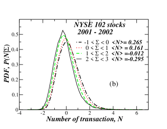
Figure 4: (a) Probability density function $P(q|\Sigma)$ of the volume of shares for given $\Sigma$. Note that $q$, $N$, and $\Sigma$ are normalized quantities with their average value subtracted. We observe that the transaction volumes are higher for groups with large $\Sigma$. (b) PDF $P(N|\Sigma)$ of $N$ for given $\Sigma$. We observe that the mean number of transaction $<N>$ slightly decreases for groups with high $\Sigma$.

To have a better understanding of how the absolute value of the price fluctuations $|R|$ effects $\Sigma,~{}\sigma,~{}q,~{}N$, we next study the PDF $P(\Sigma||R|),~{}P(\sigma||R|),~{}P(q||R|),~{}P(N||R|)$ for given $|R|$ using the TAQ database. First we sort the database of $102\times 26\times 400$ items ( 102 stocks, 26 terms per a day, about 400 days in two years) with respect to $|R|$. Next we divided these items into four groups bordered by 99.9 percentile, 99 percentile and 90 percentile. Figure 5 plots the PDF $P(\Sigma||R|),~{}P(\sigma||R|),~{}P(q||R|),~{}P(N||R|)$ of each of these groups.

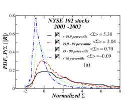
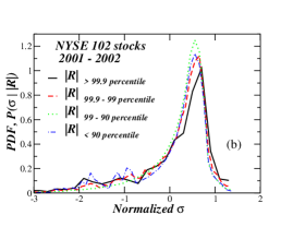
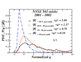
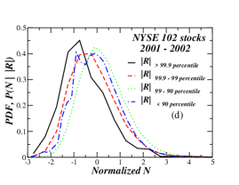
Figure 5: (a) PDF $P(\Sigma||R|)$ of $\Sigma$ for a given $|R|$. We observe that rarely occurring high $|R|$ results in higher volume fluctuations. (b) PDF $P(\sigma||R|)$ of $\sigma$ for a given $|R|$. The fluctuation of the number imbalance $\sigma$ is independent of $|R|$. (c) PDF $P(q||R|)$ of $q$ for a given $|R|$. We observe that high $|R|$ prompts the average volume of shares per trade $q$ to increase. (d) PDF $P(N||R|)$ of $N$ for a given $|R|$. We observe a slight decrease in the number of transactions with an increase in $|R|$.

We observe that even though $|R|$ is not correlated to $\Sigma$ or $q$ [c.f table 1], the PDF $P(\Sigma||R|),~{}P(q||R|)$ exhibits significant differences among different groups of $|R|$. This is because rarely occurring large $|R|$ causes large fluctuations but does not significantly contribute to correlation.

In contrast other quantities such as $\sigma$ and $N$ show there is not so much of a difference. Fig.5(d) again shows the same effect as seen in Fig.4(b) where large fluctuations decrease the number of transactions within a specified time interval.

In conclusion it can be inferred that the “two-phase behavior” as reported in Stanley1 gives no evidence as to whether critical phenomena exist in the financial market or not. The observed out of equilibrium phase is a feature of the power law PDF of the share volume. The absolute value of price fluctuation causes a large fluctuation in the share volume, and large fluctuation of the absolute price causes a decrease in the number of trades in a specified time interval.

We thank S. V. Buldyrev, Y. Lee for helpful discussions and suggestions and K. M thanks the NSF for financial support.

References

- (1) V. Plerou, P. Gopikrishnan, and H. E. Stanley. Nature, 421, 130 (2003).
- (2) X. Gabaix, P. Gopikrishnan, V. Plerou, and H. E. Stanley, Nature, 423, 267 (2003).
- (3) M. Potters. M and J. P. Bouchaud, preprint cond-mat/0304514.