Experimental verification of a one-parameter scaling law for the quantum and “classical” resonances of the atom-optics kicked rotor

Abstract

We present experimental measurements of the mean energy in the vicinity of the first and second quantum resonances of the atom optics kicked rotor for a number of different experimental parameters. Our data is rescaled and compared with the one parameter $\epsilon$–classical scaling function developed to describe the quantum resonance peaks. Additionally, experimental data is presented for the “classical” resonance which occurs in the limit as the kicking period goes to zero. This resonance is found to be analogous to the quantum resonances, and a similar one-parameter classical scaling function is derived, and found to match our experimental results. The width of the quantum and classical resonance peaks is compared, and their Sub-Fourier nature examined.

today

I Introduction

The heart of experimentally testing and controlling classical and quantum systems often lies in the introduction of an external periodic driving force LL92 ; Bayfield ; Dem . The driving probes system specific properties, the knowledge of which allows one, in turn, to understand and to optimally control the system at hand. In particular, driven systems often exhibit resonance like behavior if the external driving frequency matches the natural frequency of the unperturbed system.

Typical nonlinear classical systems are resonant for only a finite interaction time since the driving itself forces the system to gain energy and hence drift out of resonance. Only if the natural frequencies are independent of the energy as for the linear (harmonic) oscillator, can the system absorb energy on resonance indefinitely. In the quantum world, the situation may be different by virtue of the unperturbed system possibly having a discrete energy spectrum. If this spectrum shows an appropriate scaling in the excitation quantum number, resonant motion can persist forever.

A simple example of such a system is provided by the free rotor, whose energy spectrum scales quadratically in the excitation quantum number (due to periodic boundary conditions for the motion on the circle). Kicking the rotor periodically in time with a frequency commensurable with the energy difference of two neighboring levels leads to perfectly resonant driving. These so called quantum resonances of the well-studied kicked rotor (KR) Casati have been known theoretically for some time Izr , but the first traces of this example of frequency-matched driving have only recently come to light in experiments with cold atoms QRexp ; QRexpnoise . Such experiments QRexpnoise and theoretical studies sandro ; Pisa have also shown the surprisingly robust nature of these resonances in the presence of noise and perturbations.

Experimentally, the quantum resonances of the KR are hard to detect for two principle reasons. Firstly, only a relatively small proportion of atoms are kicked resonantly for the following reason: ideally, the atomic motion is along a line, which introduces an additional parameter, namely the non-integer part of the atomic momentum, i.e. the atom’s quasi-momentum. Treating the atoms independently, their motion can be mapped onto the circle owing to the spatial periodicity of the standing wave, which makes the quasi-momentum a constant of the motion. However, only some values of quasi-momentum allow resonant driving to occur Izr . All other values induce a dephasing in the evolution which hinders the resonant kicking of the atoms (see Section III for details). Secondly, if an atom is kicked resonantly it moves extremely quickly; in fact its energy grows quadratically in time (so-called ballistic propagation). These fast atoms quickly escape any fixed experimental detection window after a sufficiently large number of kicks QRexp ; QRexpnoise .

In this paper, we report experimental data which shows the behavior of a typical experimental ensemble of cold atoms under resonant driving. Our main observable is the mean energy of the atomic ensemble measured after a fixed number of kicks and scanned over the resonant kicking frequency or period. We verify a recently derived single-parameter scaling law of the resonant peak seen when scanning the energy vs. the period WGF ; WGF2 ; sandro . The scaling law allows us, for the first time, to clearly resolve the resonance peak structure because it reduces the dynamics to a stationary and experimentally robust signature of the quantum resonant motion.

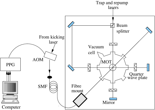
Figure 1: Schematic diagram of our experimental set up. A standard six beam magneto optical trap (MOT) of about $10^{5}$ Cs atoms is formed inside a vacuum cell at the intersection of 3 retroreflected “trapping” beams (vertical beams and (anti) Helmholtz coils are not shown). A standing wave is formed across the cloud of atoms by retroreflecting light from a “kicking laser”, which is transported to the MOT by means of a single mode fibre (SMF). This light is pulsed on and off by an acousto–optic modulator (AOM) which is gated by a programmable pulse generator (PPG). The PPG’s pulse train is uploaded from a computer, which also controls the timing of the experiment (e.g. when the trapping AOM and anti–Helmholtz coils are turned on and off).

After a short review of our experimental setup in Section II and the theoretical treatment of the atom-optics kicked rotor close to quantum resonance in Section III, we present experimental data for the mean energies around the first two fundamental quantum resonances of the kicked atom. From this data, we extract the afore mentioned scaling law in Section IV. The effect of the quasi-momentum (as a typical quantum variable) on the motion disappears in the classical limit of the kicked rotor, when the kicking period approaches zero Izr ; Fish . In the latter case, the rotor is constantly driven, and a ballistic motion occurs for all members of the atomic ensemble we . Both phenomena, the quantum and the “classical” (for vanishing kicking period) resonance are related to one another by a purely classical theory developed previously for the quantum resonance peaks WGF ; WGF2 ; sandro .

In Section V we focus on the first direct comparison of the behavior of the ensemble averaged energies in the case of the “classical” and the quantum resonance. In particular, the Sub-Fourier scaling of the resonance peaks in the mean energy as a function of the kick number is discussed. The latter makes both types of resonances studied here a potential source of high-precision measurements of system specific parameters.

II Experimental setup

Our experimental system is a realization of the paradigmatic kicked rotor (KR) model GSZ ; Moore , whose relevance lies in the fact that it shows the basic features of a complex dynamical system, and it may be used to locally (in energy) approximate much more complicated systems, such as microwave-driven Rydberg atoms IEEE , or an ion in a particle accelerator Chirikov ; LL92 .

Our experiments utilise a cloud of about $10^{5}$ cold Caesium atoms, provided by a standard six beam magneto–optical trap (MOT) Monroe1990 . The typical momentum spread of the atomic sample lies between 4 and 8 two–photon recoils. The shape of the initial momentum distribution is well approximated by a Gaussian with standard deviation $\sigma_{p}\simeq(4-8)\times 2\hbar k_{L}$, centered at zero momentum Raizen , although significant non–Gaussian tails can exist we . The width is measured in units of two–photon recoils, corresponding to the wavelength of the kicking laser $\lambda_{L}=2\pi/k_{L}$. The fractional parts in these units of the initial momenta, i.e. the quasi-momentum discussed below, are practically uniformly distributed in the fundamental Brillouin zone defined by the periodic kick potential WGF .

As shown in Fig. 1, the atoms interact with a pulsed, far-detuned optical standing wave which is created by retroreflecting the light from a 150mW (slave) diode laser which is injection locked to a lower power (master) diode laser at a wavelength of $\lambda_{L}=852\;\rm nm$. Power fluctuations were minimal during the experiments performed here ($\sim 1\%$) although larger drifts occurred over the course of many experimental runs. Accurate pulse timing is achieved using a custom built programmable pulse generator (PPG) to gate an acousto–optic modulator. The PPG is programmed by a computer running the $\rm RTLinux^{\tiny\texttrademark}$ operating system kernel RTLinuxFAQ which controls the timing of the experimental sequence (aside from the pulse train itself). Experimentally, we approximate $\delta$-kicks by pulses of width $\tau_{p}$ which are approximately rectangular in shape. The lowest value of $\tau_{p}$ used in our experiments was $240\;\rm ns$ and the highest was $480\;\rm ns$. For the experiments reported here, the effect of the finite width of the kicking pulses Raizen ; Fishman turns out to be negligible, since fairly small numbers of kicks (less than $20$) and low kicking strengths are used. In the case where the $\tau\rightarrow 0$ limit is being investigated experimentally, the $\delta$–kick assumption is clearly not valid we ; Sadgrove2005 . This restricts us to a minimum period $\tau=330\;\rm ns$, for $\tau_{p}=240\;\rm ns$, in our study of the “classical” resonance peaks.

In a typical experimental run, the cooled atoms were released from the MOT and subjected to up to 16 standing wave pulses, then allowed to expand for an additional free drift time in order to resolve the atomic momenta. After this expansion time, the trapping beam is switched on and the atoms are frozen in space by optical mollases. A CCD image of the resulting fluorescence is recorded and used to infer the momentum distribution of the atoms using standard time of flight techniques QRexp . The mean energy of the atomic ensemble may then be inferred by calculating the second moment of the experimental momentum distribution.

Kicking laser powers of up to $30\;\rm mW$ were employed, and detunings from the $6S_{1/2}(F=4)\rightarrow 6P_{3/2}(F^{\prime}=5)$ transition of Cesium of $500\;\rm MHz$ and $1\;\rm GHz$ were used for the classical and quantum resonance scans respectively. These parameters produced spontaneous emission rates of $<0.5\%$ per kick for the quantum resonance scans, which was low enough to ensure that the structure of the peaks was not affected for the low kick numbers used here.

III $\epsilon$-classical dynamics near the fundamental quantum resonances

We now consider the theoretical treatment of the atom-optics kicked rotor near quantum resonance. The Hamiltonian that generates the time evolution of the atomic wave function is (in dimensionless form) GSZ ; QRexp

$$H(t^{\prime})=\frac{p^{2}}{2}+k\cos(z)\sum_{t=0}^{N}\delta(t^{\prime}-t\tau)\;,$$ (1)

where $p$ is the atomic momentum in units of $2\hbar k_{L}$ (i.e. of two-photon recoils), $z$ is the atomic position in units of $2k_{L}$, $t^{\prime}$ is time and $t$ is an integer which counts the kicks. In our units, the kicking period $\tau$ may also be viewed as a scaled Planck constant as defined by the equation $\tau=8E_{R}T/\hbar$, where $E_{R}=\hbar^{2}k_{L}^{2}/2M$ is the recoil energy (associated with the energy change of a Caesium atom of mass $M$ after emission of a photon of wavelength $\lambda_{L}=2\pi/k_{L}=852\;\rm$nm). The dimensionless parameter $k$ is the kicking strength of the system and is proportional to the kicking laser intensity.

Figure 2: Experimentally measured mean energies around the first quantum resonance at $\tau=2\pi$ after (a) 5, (b) 10 and (c) 15 kicks. Error bars show an average over three independent experiments. The kicking strength and initial momentum standard deviation were measured to be $k=4.1\pm 0.6$ and $\sigma_{p}=5.9\pm 0.2$ respectively. Note that the estimated errors in these parameters do not take into account systematic drifts which take place over the course of experimental runs. The solid line joins the experimental points to aid the eye.

An atom periodically kicked in space and time is described by a wave packet $\psi(z)$ decomposed into $2\pi$-periodic Bloch states $\psi_{\beta}(z)$, that is,

$$\psi(z)=\int_{0}^{1}d\beta\exp(i\beta z)\psi_{\beta}(z)\,,$$ (2)

where $\beta$ is the quasi-momentum (i.e. the fractional part of momentum $p$). Quasi-momentum is conserved in the evolution generated by (1), so the different Bloch states in (2) evolve independently of each other, whereby their momenta can change only by integers by virtue of the kicks. For any given quasi-momentum, the dynamics is formally equivalent to that of a rotor (moving on a circle) whose one-period Floquet operator is given by

$${\hat{\mathcal{U}}}_{\beta}\;=\;e^{-{\rm i}k\cos({\hat{\theta}})}\;e^{-{\rm i}\tau({\hat{\mathcal{N}}}+\beta)^{2}/2},$$ (3)

where $\theta=z$mod$(2\pi)$, and ${\hat{\mathcal{N}}}=-{\rm i}d/d\theta$ is the angular momentum operator. From (3) we can immediately derive the two necessary conditions for quantum resonant motion: if $\tau=2\pi r/q$ ($r,q$ integers) then the atomic motion may show asymptotic quadratic growth in energy so long as $\beta=m/2r$, $0\leq m\leq 2r$, $m$ integer at the same time. Under these conditions the Floquet operator (3) is also periodic in momentum space, with the integer period $q$. As in previous experimental studies QRexp , we focus on the first two fundamental quantum resonances $q=1,2$, for which the amplitudes of Bloch waves with $\beta=1/2$ for $q=2$, and $\beta=0,1/2$ for $q=1$ at momentum states separated by $q\times 2\hbar k_{L}$ exactly rephase after each kick. The rephasing condition enforces ballistic propagation of the corresponding states in momentum space, so their energy grows quadratically in time. The remaining Bloch components of the original wave packet (2), with $\beta$ not in the resonant class, exchange energy with the kicking laser in a quasiperiodic manner. The competition between the resonant and the non-resonant subclasses of Bloch states (between ballistic and quasi-periodic propagation) leads to linear growth of the total mean energy, $E\approx k^{2}t/4$, obtained by incoherently averaging over the the continuous set of quasi-momenta which constitute the atomic ensemble WGF ; WGF2 ; sandro .

Figure 3: Experimentally measured mean energies around the second quantum resonance at $\tau=4\pi$ for (a) 5, (b) 10 and (c) 15 kicks. The kicking strength and initial momentum standard deviation were measured to be $k=5.0\pm 0.5$ and $\sigma_{p}=6.3\pm 0.1$ respectively. Error bars as in Fig. 2. We note both in this figure and in Fig. 2 that the resonances exhibit some asymmetry, which is thought to be of purely experimental origin (see the discussion in Section IV).

For $q=1,2$, we write $\tau=2\pi\ell+\epsilon$, where $\epsilon$ denotes the detuning from the exact resonance and $l=1,2$. As shown in WGF ; WGF2 , the Floquet operator (3), can then be rewritten as

$${\hat{\mathcal{U}}}_{\beta}(t)\;=\;e^{-{\rm i}\tilde{k}\cos({\hat{\theta}})/|\epsilon|}\;e^{-{\rm i}{\hat{\mathcal{H}}}_{\beta}/|\epsilon|}\;,$$ (4)

with $\tilde{k}=k|\epsilon|$, ${\hat{I}}=|\epsilon|{\hat{\mathcal{N}}}$ as rescaled momentum, and

$${\hat{\mathcal{H}}}_{\beta}({\hat{I}},t) = \frac{1}{2}\mbox{sign}(\epsilon){\hat{I}}^{2}+{\hat{I}}(\pi\ell+\tau\beta)\;.$$ (5)

Introducing the new variables $J=\pm I+\pi\ell+\tau\beta$, ${\vartheta}=\theta+\pi(1-\mbox{\rm sgn}(\epsilon))/2$, where $\pm$ denotes the sign of $\epsilon$ $=\mbox{sign}(\epsilon)$, the quantum evolution can be approximated by the $\epsilon$-classical Standard Map derived in WGF ; WGF2 ; como

$$J_{t+1}=J_{t}+{\tilde{k}}\sin(\vartheta_{t+1})\;\;,\;\;\vartheta_{t+1}=\vartheta_{t}+J_{t}\;,$$ (6)

for ${\tilde{k}}\ll 1$. $J_{t}$ implicitly contains the quasi-momentum $\beta$, which defines the initial conditions in momentum in the phase space generated by the map (6) sandro .

For small $|\epsilon|$, the $\epsilon-$classical dynamics is quasi-integrable, and the growth of the energy is dominated by the principal $\epsilon-$classical resonant island around $J=2\pi$ LL92 . The latter island is populated only by the values of $\beta$ which are close to the resonant ones, whilst the non-resonant quasi-momenta correspond to initial conditions outside the nonlinear resonance island sandro ; WGF ; WGF2 . Moreover, at any time $t$, the ratio between the energy and its value at $\epsilon=0$ is a scaling function of the single variable

$$x=t\sqrt{k|\epsilon|}.$$ (7)

The scaling function (which was explicitly derived in WGF ; WGF2 ; sandro ) is

$$\frac{\langle E_{t,\epsilon}\rangle}{\langle E_{t,0}\rangle}\approx R(x)\equiv 1-\Phi_{0}(x)+\frac{4}{\pi x}G(x)\;,$$ (8)

with the functions

$$\Phi_{0}(x)\equiv\frac{2}{\pi}\int_{0}^{x}ds\;\frac{\sin^{2}(s)}{s^{2}}\;,$$

and

$$G(x)\approx\frac{1}{8\pi}\int_{0}^{2\pi}{\rm d}\theta_{0}\int_{-2}^{2}{\rm d}J_{0}\overline{J}(x,\theta_{0},J_{0})^{2}\;.$$

$\overline{J}\equiv J/\sqrt{{\tilde{k}}}$ is the momentum of the pendulum approximation to the dynamics generated around the stable fixed point of (6), rescaled to unit coupling parameter (see WGF ; WGF2 ; sandro for details).

The one-parameter scaling law (8) allows us to deduce the shape and the parameter dependence of the resonance peaks elegantly from the experimental data, which in the unscaled form is shown in the Figs. 2 and 3 for $\tau=2\pi$ and $\tau=4\pi$, respectively.

IV Experimental verification of the scaling law at quantum resonance

Figure 4: Experimental mean energies around $\tau=2\pi$ taken from Fig. 2 and rescaled as $(\langle E_{t,\epsilon}\rangle-\sigma_{p}^{2}/2)/(tk^{2}/4)$. Triangles are for $t=5$, squares for $t=10$ and circles for $t=15$. Error bars represent statistical fluctuations over three experiments, and do not take into account fluctuations in $k$ or $\sigma_{p}$. The solid line shows the numerically evaluated scaling function $R(x)$ of Eq. (8). We note that, for 10 and 15 kicks, data for $|\epsilon|<0.03$ has been omitted due to our inability to accurately resolve atomic energies for fast atoms this close to resonance. Experimental data for both positive and negative values of $\epsilon$ is plotted. We would like to note the good correspondence between the $\epsilon$-classical prediction and the experimental data for over one order of magnitude in the scaling variable $x$.

We have used the data obtained for various scans of the mean energy vs. the kicking period around the quantum resonances $\tau=2\pi$ and $\tau=4\pi$, and for kick numbers $t=5,10,15$ to extract the ratio $\frac{\langle E_{t,\epsilon}\rangle}{\langle E_{t,0}\rangle}$. We subtract from the numerator the initial energy of the atomic ensemble with the characteristic width in momentum space $\sigma_{p}$. The contribution of $\sigma_{p}^{2}/2$ to the energy must be subtracted because the derivation of the scaling function $R(x)$ assumed an initial atomic momentum distribution in the unit interval $[0,1)$ WGF , corresponding to a uniform distribution of quasi-momenta $\beta\equiv p_{0}\in[0,1)$. Since the maximum of the resonance peak $\langle E_{t,\epsilon=0}\rangle$ is experimentally the most unstable parameter (due to the early loss of the fastest resonant atoms from the experimental detection window QRexp ; QRexpnoise ; sandro ), we use the theoretical value $\langle E_{t,0}\rangle-\sigma_{p}^{2}/2=k^{2}t/4$ to rescale our experimental data, rather than the height of the experimental peak itself. Results are presented in Figs. 4 and 5 for $\tau=2\pi,4\pi$ respectively. We see very good agreement between the theoretical scaling function $R(x)$ from Eq. (8) and our experimental data. Despite the relatively large experimental errors due to the uncertainty in the determination of $\sigma_{p}$ (see discussion below), the data shows the characteristic structure, and also the oscillations arising from the contribution of the function $G(x)$ at large $x\geq 8$. These oscillations arise from the averaged contributions of the initial conditions $\overline{J}_{0}\in(-2,2)$ within the principal nonlinear resonance island, which evolve with different frequencies around the corresponding elliptic fixed point of the map (6). The quasi-momentum classes contributing to $G(x)$ are thus the near-resonant values, whilst the non-resonant values contribute to the function $1-\Phi_{0}(x)$, which saturates to a constant for large $x$ WGF ; WGF2 ; sandro .

We fitted $k$ and $\sigma_{p}$ for each data set and then used these fitted parameters to scale our data. In the case of the $\tau=2\pi$ data, the best fit value of $k$ was found to be $4.5$ compared to the independently measured value of $k=4.1\pm 0.6$. For the $\tau=4\pi$ data, the best fit value of $k$ was $5.2$ compared with a measured value of $k=5\pm 0.5$. The corresponding fitted values of $\sigma_{p}$ were $5$ and $5.2$ two–photon recoils respectively which differ from the measured values of $4.53\pm 0.02$ and $4.3\pm 0.2$. This difference is due to the systematic error involved in determining $\sigma_{p}$ from the experimental initial momentum distribution (as discussed in we ). In particular this distribution may have noisy exponential wings Raizen which must truncated in order to reliably extract the second moment leading to an underestimation of the true initial momentum spread.

It is interesting to note that in Figs. 2 and 3, there is noticeable asymmetry in the resonance peaks. This degree of asymmetry is not predicted by the standard $\epsilon$–classical theory and its precise cause has not yet been ascertained. However, the asymmetry most likely stems from one or more systematic experimental effects, including the effect of small amounts of spontaneous emission ($<0.5\%$ chance per kick for the quantum resonance scans) and also from the slightly lesser time of flight experienced by atoms for positive as opposed to negative $\epsilon$. Asymmetry of the peaks has also been noted in other experiments probing the structure of the quantum resonances hoogerland . In any case, this asymmetry does not prevent us from observing the structure of the quantum resonances, but leads to a slightly enhanced scatter of the experimental data points in Figs. 4 and 5.

Figure 5: Scaled experimental mean energies around $\tau=2\pi$ taken from Fig. 3; triangles are for $t=5$, squares for $t=10$ and circles for $t=15$ kicks. The solid line shows the scaling function $R(x)$ from Eq. (8). Again, for 10 and 15 kicks, data too close to resonance, i.e. for $|\epsilon|<0.03$, has been omitted.

V Classical limit of vanishing kicking period

In spite of the intrinsically quantum nature of the quantum resonances as an example of perfectly frequency-matched driving, the method reviewed in Section III allows us to map the quantum dynamics onto a purely classical map given by (6). The latter map is formally equivalent to the usual Standard Map, which describes the classical limit of the quantum KR when the kicking period tends to zero Fish :

$$J_{t+1}=J_{t}+{\tilde{k}}\sin(\theta_{t+1})\;\;,\;\;\theta_{t+1}=\theta_{t}+J_{t}\;,$$ (9)

now with $J=\tau p=\tau(n+\beta)$, and ${\tilde{k}}=k\tau$. Because of the analogy between the maps (6) and (9), we expect a scaling law for the mean energy also in the limit $\tau\to 0$. Since $\tau\to 0$, all quasi-momentum subclasses contribute now similarly to the energy growth, and the averaged energy is given only by the initial conditions within the principal nonlinear resonance island (see we for details):

$$\langle E_{t,\tau}\rangle\approx\tau^{-2}\langle(J_{t})^{2}\rangle/2\approx k/2\tau G_{cl}(x),$$ (10)

with

$$G_{cl}(x) \equiv \frac{\sqrt{k}}{2\pi\sqrt{\tau}}\int_{0}^{2\pi}{\rm d}\theta_{0}\int_{0}^{\sqrt{\tau/k}}{\rm d}J_{0}\overline{J}(x,\theta_{0},J_{0})^{2}$$ (11)

$$\approx \frac{1}{2\pi}\int_{0}^{2\pi}{\rm d}\theta_{0}\overline{J}(x,\theta_{0},J_{0}=0)^{2}\;,$$

which depends on the variable $x=t(k\tau)^{1/2}$ (which, given that $\tau=\epsilon$ for the classical resonance, is the same as the scaling variable given in Eq. (7)) and weakly on $k$ and $\tau$, in contrast to the quantum resonant case studied in Section III. The dependence of $G_{cl}$ on $\tau$ is negligibly small for $\tau\lesssim 1/k$, so that practically, $G_{cl}$ can be viewed as a function of the scaling parameter $x$ alone.

For the ratio $\langle E_{t,\tau}\rangle/\langle E_{t,0}\rangle$ we then arrive at the scaling function

$$\frac{\langle E_{t,\tau}\rangle}{\langle E_{t,0}\rangle}\approx R_{cl}(x)\equiv\frac{2}{x^{2}}G_{cl}(x)\;,$$ (12)

which in the limit of vanishing $\tau$ tends to unity, since $G_{cl}(x)\approx x^{2}/2$ for small $x$ we ; sandro . Our result (10) describes quadratic growth in mean energy as $\tau\to 0$. We note again that in the case of quantum resonances, $\epsilon$-classical theory predicts only linear mean energy growth with kick number at quantum resonance WGF ; WGF2 . This linear increase is induced by the contribution of most quasi-momentum classes which lie outside the classical resonance island. For $\tau\to 0$, almost all initial conditions (or quasi-momenta) lie within the principal resonance island, which leads to the ballistic growth for the averaged ensemble energy (10).

For finite $\tau>0$ and $t^{2}k\gg 1/\tau$, we obtain from (10)

$$\langle E_{t,\tau>0}\rangle\approx\frac{k}{2\tau}\alpha\;,$$ (13)

since $G_{cl}$ saturates to the value $\alpha\simeq 0.7$ for large $x$. Within the stated parameter range, this result implies dynamical freezing – the ensemble’s mean energy is independent of kick number. This phenomenon is a classical effect in a system with a regular phase space, and has been observed in we for the first time. It is distinct from dynamical localization which is the quantum suppression of momentum diffusion for a chaotic phase space Casati ; Fish . Experimentally, the freezing effect corresponds to the cessation of energy absorption from the kicks, similar (but different in origin) to that which occurs at dynamical localization. The freezing may be explained as the averaging over all trajectories which start at momenta close to zero, and move with different frequencies about the principal elliptic fixed point of the map (9).

From Eq. (12), we immediately see that for the “classical” resonance $\tau\to 0$, the resonant peak width scales in time like $(kt^{2})^{-1}$, as at the quantum resonances studied in Sections III and IV. However, the tails of the classical resonance peak decay faster (as $\propto 1/x^{2}$) than those at quantum resonance (as $\propto 1/x$, c.f. Eq. (8)). This very fast shrinking of both types of resonance peaks is compared in Figs. 6 and 7.

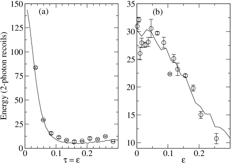
Figure 6: (a) Circles show experimentally measured mean energies as $\tau\rightarrow 0$ after 5 kicks. The measured value of $k$ is $4.9\pm 0.2$. The solid line is classical data for $k=4.9$, as generated by the map (9), using practically the same initial momentum distribution as in the experiment. The thermal energy $\sigma_{p}^{2}/2$ has been subtracted to facilitate comparison with the quantum resonance curve in (b). In (b), circles show experimental data after 5 kicks near the second quantum resonance for positive $\epsilon=\tau-4\pi$ and the experimental parameters are as given for Fig. 3. The thermal energy $\sigma_{p}^{2}/2$ has been subtracted. The solid line is $\epsilon$–classical data as generated by the map (6).

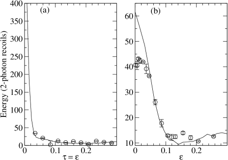
Figure 7: (a) Circles show experimental data as $\tau\rightarrow 0$ for 10 kicks. The other experimental parameters are the same as those given for Fig. 6(a). The circles in (b) show experimental data once again for the second quantum resonance after 10 kicks this time. Other experimental parameters are the same as those given for Fig. 6(b). We note that for the quantum resonance in (b), the simulation and experimental results differ most markedly near the resonance peak. In this region ($\epsilon\lesssim 0.03$), some fast, resonant atoms are being lost from the experimental viewing area leading to a lower energy growth rate than predicted theoretically (see discussion in Sections I and II). Note that in (a), it is not possible to probe low values of $\tau=\epsilon$ due to the finite width of the pulses.

Both types of these sensitive resonance peaks may serve as an experimental tool for determining or calibrating parameters in a very precise manner. Additionally, we note that the quadratic scaling in time at the quantum resonances and the “classical” resonance, respectively, is much faster and hence much more sensitive than the Sub-Fourier resonances detected in a similar context by Szriftgizer and co-workers Lille . A detailed study of the quantum energy spectrum of the kicked atoms close to the two types of resonances is under way to clarify the origin of the observed Sub-Fourier scaling of the resonance peaks.

Finally, we have plotted rescaled experimental data for the $\tau\rightarrow 0$ resonance against the scaling function of Eq. (12), as seen in Fig. 8. The scaling was performed using the fitted parameters as given in Figs. 6 and 7. We note that it is more difficult to extract the scaling from experimental data in the classical case, as opposed to the quantum case, because the peak of the extremely narrow resonance is difficult to probe. This leads to a larger uncertainty in the scaled energy and the points appear somewhat more scattered than those in Figs. 4 and 5. However, the points clearly agree much better with the classical scaling function from (12) than the $\epsilon$-classical scaling function (8) which is shown in Fig. 8 as a dash-dotted line. The clearly different scaling of the quantum and the “classical” resonant peaks goes along with the same rates at which the peaks become narrower with time in a Sub-Fourier manner.

VI Conclusions

Figure 8: Rescaled experimental mean energies for $\tau=0.034\ldots 0.284$ (corresponding to $0.33\ldots 2.75\;\rm\mu s$). The data is for $k=4.9$ with $t=3$ (circles), $t=7$ (diamonds) and $t=16$ (stars). Error bars indicate statistical fluctuations over three experiments, and do not include variations in $k$ or $\sigma_{p}$. The solid line shows the classical scaling function of Eq. (12). The dash-dotted line shows the scaling function from Eq. (8) (valid for the quantum resonances) for comparison.

In summary, we have experimentally confirmed a theoretically predicted one-parameter scaling law for the resonance peaks in the mean energy of a periodically kicked cold atomic ensemble. This scaling of the resonant peaks is universal, in the sense that it reduces the dependence from all the system’s parameters to just one combination of such variables. Furthermore, the scaling theory works in principle for arbitrary initial momentum distributions. In particular, it is valid for the experimentally relevant uniformly distributed quasi-momenta at the fundamental quantum resonances of the kicked atoms. In the classical limit of vanishing kicking period, the dependence on quasi-momentum, as an intrinsic quantum variable, disappears entirely, leading to a simpler version of the scaling law. The discussed scaling of the experimental data offers one the possibility to clearly observe the quantum and “classical” resonant peak structure over more than one order of magnitude in the scaling variable. Furthermore, its sensitive dependence on the system’s parameters may be useful for high-precision calibration and measurements.

It will be of great interest to clarify whether a similar universal scaling law can be found for other time-dependent systems, such as the close–to–resonant dynamics of the kicked harmonic oscillator QKHO , or the driven Harper model Harpertheo1 ; Harpertheo2 . As with the atom-optics kicked rotor, both of the latter systems may be readily realized in laboratory experiments Harperexp ; Zoller .

Acknowlegements

M.S. thanks T. Mullins for his assistance in the laboratory prior to these experiments and acknowledges the support of a Top Achiever Doctoral Scholarship, 03131.

S.W. warmly thanks Prof. Ennio Arimondo and PD Dr. Andreas Buchleitner for useful discussions and logistical support, and acknowledges funding by the Alexander von Humboldt Foundation (Feodor-Lynen Fellowship) and the Scuola di Dottorato di G. Galilei della Università di Pisa.

References

- (1) A.L. Lichtenberg and M.A. Lieberman, Regular and Chaotic Dynamics, (Springer, Berlin, 1992).
- (2) J. E. Bayfield, Quantum Evolution: An Introduction to Time-Dependent Quantum Mechanics, (Wiley, New-York, 1999).
- (3) W. Demtröder, Laser Spectroscopy: Basic Concepts and Instrumentation, (Springer, Berlin, 2003).
- (4) G. Casati et. al., in Stochastic Behavior in Classical and Quantum Hamiltonian Systems, ed. by G. Casati and J. Ford (Springer, Berlin, 1979), p. 334.
- (5) F.M. Izrailev and D.L. Shepelyansky Sov. Phys. Dokl. 24, 996 (1979); F.M. Izrailev, Phys. Rep. 196, 299 (1990).
- (6) W.H. Oskay et al., Opt. Comm. 179, 137 (2000); M.E.K. Williams et al., J. Opt. B: Quantum Semiclass. Opt. 6, 28 (2004); G. Duffy et al., Phys. Rev. E 70, 056206 (2004).
- (7) M.B. d’Arcy et al., Phys. Rev. Lett. 87, 074102 (2001); M.B. d’Arcy et al., Phys. Rev. E 69, 027201 (2004); M. Sadgrove et al., ibid. 70, 036217 (2004).
- (8) S. Wimberger, Ph.D. Thesis, University of Munich and Università degli Studi dell’ Insubria (2004), available at http://edoc.ub.uni-muenchen.de/archive/00001687/.
- (9) S. Wimberger, R. Mannella, O. Morsch, and E. Arimondo, cond-mat/0501565; L. Rebuzzini, S. Wimberger, and R. Artuso, nlin.CD/0410015.
- (10) S. Wimberger, I. Guarneri, and S. Fishman, Nonlinearity 16, 1381 (2003).
- (11) S. Wimberger, I. Guarneri, and S. Fishman, Phys. Rev. Lett. 92, 084102 (2004).
- (12) S. Fishman, in Quantum Chaos, School “E. Fermi” CXIX, eds. G. Casati et al. (IOS, Amsterdam, 1993).
- (13) M. Sadgrove, S. Wimberger, S. Parkins, and R. Leonhardt, submitted to Phys. Rev. Lett.
- (14) R. Graham, M. Schlautmann, and P. Zoller, Phys. Rev. A 45, R19 (1992).
- (15) F.L. Moore et al., Phys. Rev. Lett. 75, 4598 (1995).
- (16) G. Casati, I. Guarneri, and D. Shepelyansky, IEEE J. Quantum Electron. 24, 1420 (1988); S. Wimberger and A. Buchleitner, J. Phys. A 34, 7181 (2001).
- (17) B.V. Chirikov, Phys. Rep. 52, 263 (1979).
- (18) C. Monroe, W. Swann, H. Robinson and C. Wieman, Phys. Rev. Lett. 65, 1571 (1990)
- (19) B.G. Klappauf, W.H. Oskay, D.A. Steck, and M.G. Raizen, Physica D 131, 78 (1999).
- (20) FSMLabs Inc., http://www.fsmlabs.com/products/rtlinuxpro/rtlinuxpro_faq.html.
- (21) M. Sadgrove, T. Mullins, S. Parkins and R. Leonhardt, Phys. Rev. E 71, 027201 (2005).
- (22) R. Blümel, S. Fishman, and U. Smilansky, J. Chem. Phys. 84, 2604 (1986).
- (23) S. Fishman, I. Guarneri, and L. Rebuzzini, J. Stat. Phys. 110, 911 (2003); Phys. Rev. Lett. 89, 084101 (2002).
- (24) M. Hoogerland, S. Wayper, and W. Simpson, unpublished.
- (25) P. Szriftgiser, J. Ringot, D. Delande, and J. C. Garreau, Phys. Rev. Lett. 89, 224101 (2002); H. Lignier, J. C. Garreau, P. Szriftgiser, and D. Delande, Europhys. Lett. 69, 327 (2005).
- (26) G.M. Zaslavsky et al., Weak chaos and quasi-regular patterns (Cambridge Univ. Press, 1992); D. Shepelyansky, C. Sire, Europhys. Lett. 20, 95 (1992); F. Borgonovi and L. Rebuzzini, Phys. Rev. E 52, 2302 (1995); A.R.R. Carvalho and A. Buchleitner, Phys. Rev. Lett. 93, 204101 (2004).
- (27) P. Leboeuf, J. Kurchan, M. Feingold, and D. P. Arovas, Phys. Rev. Lett. 65, 3076 (1990); T. Geisel, R. Ketzmerick, and G. Petschel ibid. 66, 1651 (1991); R. Artuso et. al., ibid. 69, 3302 (1992); I. Guarneri and F. Borgonovi, J. Phys. A 26, 119 (1993); I. Dana, Phys. Rev. E 52, 466 (1995).
- (28) O. Brodier, P. Schlagheck, and D. Ullmo, Phys. Rev. Lett. 87, 064101 (2001); A. R. Kolovsky and H. J. Korsch, Phys. Rev. E 68, 046202 (2003).
- (29) H.-J. Stöckmann, Quantum chaos: an introduction (Cambridge University Press, Cambridge, 1999); T.M. Fromhold et. al., Nature 428, 726 (2004).
- (30) S.A. Gardiner, J.I. Cirac, and P. Zoller, Phys. Rev. Lett. 79, 4790 (1997); S.A. Gardiner et. al., Phys. Rev. A 62, 023612 (2000).