Phase distortion mechanisms in
linear beam vacuum devices

Abstract

The mechanism for phase distortion in linear beam vacuum devices is identified in the simplest system that pertains to such devices, the force-free drifting electron beam. We show that the dominant cause of phase distortion in a force-free drifting beam is the inverse dependence of arrival time on velocity for an electron, i.e., the “$1/u$ nonlinearity,” and that a secondary cause of phase distortion is the nonlinearity of the velocity modulation. We claim that this is the mechanism for phase distortion in all linear beam vacuum devices, and provide evidence from a traveling wave tube calculation. Finally, we discuss the force-free drifting beam example in the context of the “self-intermodulation” description of phase distortion recently described in Refs. [J. Wöhlbier and J. Booske, Phys. Rev. E, vol. 69, 2004, 066502], [J. Wöhlbier and J. Booske, IEEE Trans. Elec. Devices, To appear.]

We recently reported on mechanisms for phase distortion in linear beam vacuum devices [3, 4]. The mechanism for phase distortion was reported there as a “self-intermodulation” process, where harmonic beam distortions interacted with the fundamental beam modulation to produce a phase shift at the fundamental. While this frequency domain view of phase distortion is a useful one, we felt that a corresponding time domain view of phase distortion would be a useful contribution to the overall understanding of phase distortion. In this note we consider the simplest possible system that pertains to linear beam electron devices, a space charge free (“force-free”) drifting electron beam. Indeed the physical mechanism for phase distortion exists in the force-free drifting beam, and hence the system provides the most lucid example in which to study phase distortion.

A 1-d force-free drifting beam is described by Burger’s equation for the beam velocity $u$,

$$u_{t}+uu_{x} = 0,$$ (1)

where $x$ is space, $t$ is time, and the subscripts indicate partial derivatives. To apply Eq. (1) to a klystron where the space charge force is negligible, for example, one sets the boundary value of $u$ as the sum of a dc beam velocity $u_{0}$ and a sinusoidal perturbation due to the cavity modulation. Assuming that the dc velocity is normalized to $1$, this is written

$$u(0,t) = 1+\epsilon\sin{\omega t}.$$ (2)

Given the solution to Eq. (1) with boundary condition (2), the beam density evolution is obtained by solving the continuity equation

$$\rho_{t}+(\rho u)_{x} = 0$$ (3)

for an appropriate density boundary condition.

The force-free Burger’s equation (1) implies that the velocity of an electron (fluid element) does not change, i.e., the $(x,t)$ trajectories, or characteristics, of Eq. (1) are straight lines with slopes determined by the boundary data. In vacuum electronics the density bunching that results from the sinusoidal velocity modulation is called “ballistic bunching.” Initially we will consider inputs for which there is no electron overtaking, and inputs such that electron overtaking occurs will be considered later.

In principle the force-free drifting electron beam can be solved exactly prior to electron overtaking, although closed form analytic solutions need to be written in terms of infinite series [1]. Equation (1) is solved using the method of characteristics. The method of characteristics involves changing the equations to Lagrangian independent coordinates (material coordinates), solving the equations in Lagrangian coordinates, and changing the solution back to Eulerian coordinates. For a fluid element that crosses $x=0$ at time $t_{0}$ we write the transformation from Lagrangian to Eulerian coordinates as the time function $t(x,t_{0})$, i.e., the time fluid element $t_{0}$ arrives at $x$, with $t(0,t_{0})=t_{0}$. Since the velocity is a constant for each fluid element, the velocity solution in Lagrangian coordinates is

$$u(x,t_{0}) = 1+\epsilon\sin{\omega t_{0}}.$$ (4)

That is, independent of location $x$, the velocity of an electron is set by the time $t_{0}$ at which it crosses $x=0$. Since the electron orbits are straight line trajectories in $(x,t)$ space, we can infer the solution for the function $t(x,t_{0})$

$$t(x,t_{0}) = t_{0}+\frac{x}{u(x,t_{0})}$$ (5)

$$= t_{0}+\frac{x}{1+\epsilon\sin{\omega t_{0}}}.$$ (6)

To solve for $u(x,t)$ one needs to invert the function $t(x,t_{0})$, i.e., calculate $t_{0}(x,t)$, and substitute it into Eq. (4). Since we restrict, for now, our attention to input levels such that no electron overtaking occurs, i.e., the characteristics do not cross, Eq. (6) can be inverted. Unfortunately $t(x,t_{0})$ in Eq. (6) is a transcendental function of $t_{0}$, so an analytic inverse needs to be expressed in terms of an infinite series.

For phase distortion we are ultimately interested in the beam current and beam density, since they linearly drive circuit or cavity fields. The continuity equation in Lagrangian coordinates is given by [5, 1]

$$\rho(x,t_{0}) = \frac{\rho(0,t_{0})u(0,t_{0})}{\left|\frac{\partial t\hfill}{\partial t_{0}}\right|u(x,t_{0})}$$ (7)

$$= \frac{\rho(0,t_{0})}{\left|\frac{\partial t\hfill}{\partial t_{0}}\right|}$$ (8)

where the last equality comes from the fact that $u(0,t_{0})=u(x,t_{0})$ since we are considering a force-free drifting beam. For the density solution in Eulerian coordinates one composes the density in Lagrangian coordinates (8) with the mapping from Eulerian to Lagrangian coordinates $t_{0}(x,t)$.

The factor $\partial t/\partial t_{0}$ is the Jacobian of the transformation from Lagrangian to Eulerian coordinates, and it quantifies the amount of stretching or compressing in time the electron beam undergoes. That is, for a fluid element entering the system of time length $\delta t_{0}$, it will occupy a time length of $\delta t=(\partial t(x,t_{0})/\partial t_{0})\delta t_{0}$ downstream at position $x$. For purposes of explaining phase distortion it will be convenient to write the Jacobian in terms of derivatives with respect to both $t_{0}$ and $u$, i.e.,

$$\frac{\partial t\hfill}{\partial t_{0}} = \frac{\partial\hat{t}\hfill}{\partial t_{0}}+\frac{\partial\hat{t}}{\partial u\hfill}\frac{\partial u\hfill}{\partial t_{0}}.$$ (9)

In Fig. 1 we show density solutions versus time, where a root finder was used to invert Eq. (6).

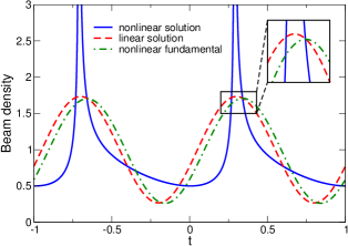
Figure 1: Nonlinear, linear, and fundamental component of nonlinear density solution versus $t$ at $x=0.3$ for two periods.

The results are for the velocity modulation (2) with $\omega=2\pi$ and a uniform density boundary condition $\rho(0,t_{0})=1$. To accentuate the effect of phase distortion we use a strong velocity modulation, $\epsilon=0.389$, and observe the output at $x=0.3$. There is no electron overtaking at $x$ if the Jacobian stays greater than zero, i.e., when

$$x\frac{\epsilon\omega\cos\omega t_{0}}{\left(1+\epsilon\sin\omega t_{0}\right)^{2}} \leq 1$$ (10)

for all $t_{0}$. In the present case the maximum value of the left hand side of Eq. (10) is equal to $0.9992$ with $x=0.3$. The linear velocity and density solutions are solutions to the (normalized) linear equations

$$u_{t}+u_{x} = 0$$ (11)

$$\rho_{t}+\rho_{x}+u_{x} = 0$$ (12)

and, for the same boundary data as used for the nonlinear problem, are given by

$$u_{\rm lin}(t,x) = 1+\epsilon\sin\omega(t-x)$$ (13)

$$\rho_{\rm lin}(t,x) = 1+x\epsilon\omega\cos\omega(t-x).$$ (14)

In Fig. 1 the nonlinear density solution, the linear density solution, and the fundamental component of the nonlinear density solution obtained by using a fast Fourier transform are shown. The phase shift between the linear density solution and the fundamental component of the nonlinear density solution is the “phase distortion” of the nonlinear solution. It is clear from the figure that the reason for the phase shift of the fundamental component of the nonlinear density solution from the linear solution is because the density is larger “on average” behind (in time) the density peak (early times are to the left). Therefore, to explain phase distortion one must explain the reason for the asymmetry in the density about the density peak. (Also note that for this value of $\epsilon$ the nonlinear solution shown in Fig. 1 shows “amplitude distortion” in that the fundamental component of the density is smaller than the predicted linear density amplitude.)

The reason for the the higher density behind the peak comes predominantly from the “$1/u$ nonlinearity” in the arrival time function (5), and secondarily from the nonlinearity of the $\epsilon\sin\omega t_{0}$ velocity modulation. It is intuitive that about a larger initial velocity $u$, a given deviation $\pm\delta u$ will result in a smaller $\mp\delta t$ at $x$ than the same $\pm\delta u$ would have on $\mp\delta t$ for a smaller initial velocity $u$ [a fluid element with velocity $u\pm\delta u$ arrives earlier (later), at time $t\mp\delta t$, than a fluid element with velocity $u$ which arrives at $t$]. This intuition is of course borne out by the derivative

$$\frac{\partial t}{\partial u} = -\frac{x}{u^{2}}$$ (15)

evaluated at large and small values of velocity $u$. This dependence causes phase distortion in that relatively slower fluid elements stretch and compress differently than the relatively faster fluid elements. That is, the size of density fluctuations at a fluid element depends on its initial velocity, with smaller initial velocities having larger fluctuations. This effect is best demonstrated with an example where more specific points regarding the interplay of the $1/u$ nonlinearity and the nonlinearity of the velocity modulation may be emphasized.

In Fig. 2 we show the velocity modulation, the Jacobian, and the density versus fluid element $t_{0}$ at $x=0.3$.

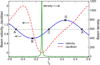
Figure 2: Beam velocity, beam density, and Jacobian versus fluid element label $t_{0}$ at $x=0.3$. That is, the value of velocity, density and Jacobian that the fluid element that crossed $x=0$ at time $t_{0}$ will have when it arrives at $x=0.3$. Results show slightly more than one period in $t_{0}$.

Note that since $u(x,t_{0})=u(0,t_{0})$ the velocity versus fluid element label $t_{0}$ is also the initial velocity modulation at $x=0$ versus fluid element label $t_{0}$. In the region B–D the beam is bunched because fluid elements entering at any time are given a faster initial velocity than the fluid elements entering just prior to them, where again we assume for the time being that modulations are not strong enough to cause electron overtaking. It is instructive to look at the expression for the Jacobian,

$$\frac{\partial t\hfill}{\partial t_{0}} = 1+\frac{\partial t}{\partial u}\frac{\partial u\hfill}{\partial t_{0}},$$ (16)

and determine, for example, the fluid element at which the density will be maximum. The Jacobian is inversely proportional to density, and hence the maximum density occurs the minimum Jacobian; for a given $\delta t_{0}$ the minimum $\delta t$ corresponds to the maximum fluid compression. Consider the two derivatives on the right hand side of Eq. (16). As described above, due to the inverse dependence of $t$ on $u$, for a given $\delta u$ fluid elements with relatively larger initial velocities in B–D will be compressed less than fluid elements with relatively smaller initial velocities. That is, $\partial t/\partial u$ is largest negative at B and smallest negative at D. Furthermore, for the sinusoidal velocity modulation the change in velocity for a given $\delta t_{0}$, $\partial u/\partial t_{0}$, is zero at point B and increases to a maximum at point C. The minimum Jacobian will occur at a fluid element between points B and C such that $(\partial t/\partial u)(\partial u/\partial t_{0})$ is the largest negative. The value of $t_{0}$ for which this happens can be computed by setting the derivative of the Jacobian with respect to $t_{0}$ to zero, and solving for $t_{0}$. For the linear solution point C is the fluid element around which the density is maximum.

The density asymmetry about the peak also comes from the $1/u$ nonlinearity. Since the compression is enhanced in B–C relative to C–D, region B–C becomes smaller than C–D, as seen in Fig. 3. The results in Fig. 3 are the solutions in Eulerian coordinates which are obtained by composing the Lagrangian solutions in Fig. 2 with the map $t_{0}(x,t)$, i.e., the mapping that determines which fluid element $t_{0}$ arrives at a given $(x,t)$, shown in Fig. 4.

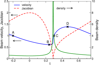
Figure 3: Beam velocity, density, and Jacobian versus $t$ at $x=0.3$ for one period of $t$. Results are those of Fig. 2 composed with $t_{0}(x,t)$. shown in Fig. 4.

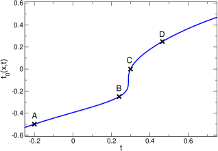
Figure 4: Mapping $t_{0}(x,t)$ from Eulerian to Lagrangian coordinates at $x=0.3$ for one period of $t$.

Indeed while the maximum density fluid element lies nearly half way between points B and C at the input (see Fig. 2) it is very near to point C by $x=0.3$, the point about which the linear density is maximum, as seen in Fig. 3. Because B–C is much more compressed than C–D, loosely speaking, the regions that neighbor the region of maximum density are a stretched region A–B earlier in time and the compressed region C–D along with the stretched region D–A (periodic waveform) later in time. Furthermore, the stretched region A–B has enhanced stretching over region D–A, contributing to the higher density behind (in time) the peak.

In sum, the above describes how phase distortion of a force-free drifting beam is a manifestation primarily of the inverse dependence of the arrival time $t(x,t_{0})$ on velocity $u$, but also depends on the nonlinearity of the velocity modulation. To prove that the “dominant” cause for phase distortion is the $1/u$ nonlinearity we do the following calculation. First, for a small velocity modulation ($\epsilon$ small) we can linearize the $1/u$ nonlinearity to get

$$t(x,t_{0}) \approx t_{0}+x(1-\epsilon\sin\omega t_{0}),$$ (17)

$$\frac{\partial t\hfill}{\partial t_{0}} \approx 1-x\epsilon\omega\cos\omega t_{0}.$$ (18)

For this arrival time function the location of maximum density (minimum Jacobian) is the same as for the linear solution, point C in Fig. 3. However, with this approximation the problem does not immediately reduce to the linear solution since the characteristics do not all have the same slope. In this limit there is no phase distortion since Eq. (18) is an even function about the Jacobian minimum, and hence the density is an even function about the density peak. Furthermore, we could replace the modulation by any periodic function that is odd in $t_{0}$ (plus or minus an arbitrary time shift) for a period and get the same result. Thus, by linearizing the $1/u$ nonlinearity and not linearizing the velocity modulation the phase distortion is removed. This confirms that the $1/u$ nonlinearity is the dominant cause of phase distortion.

Up to now we have restricted the input to a level such that electron trajectories do not cross. The reason for such a restriction was to ensure that the phase distortion physics was not potentially clouded by electron overtaking physics. In fact, no such restriction was necessary, and the principle of phase distortion is the same even when the input is set such that electron trajectories cross. In Fig. 5 we show the beam velocity, nonlinear

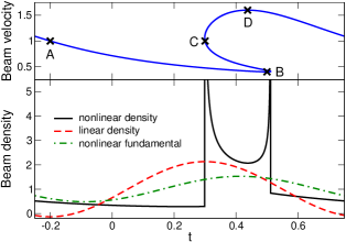
Figure 5: Nonlinear beam density, linear beam density, fundamental component of the nonlinear beam density, and nonlinear beam velocity for an input such that electron overtaking occurs.

beam density, linear beam density, and the fundamental component of the nonlinear beam density for an input of $\epsilon=0.6$. The velocity solution and the two peaked structure of the density confirm the multi-valued nature of the solutions. From the fluid element labels we see that region B–D is in the multi-phase region of the density, and that the higher density behind the peak is again because region D–A (or region B–A outside the multi-phase zone) is not stretched to the extent that region A–B (or region A–C outside the multi-phase zone) is.

Even though the preceding analysis considered only a force-free drifting beam, we claim that phase distortion mechanism identified holds more generally for klystrons when space charge forces are considered, and in traveling wave tubes (TWTs). The reason is again the inverse dependence of arrival time on velocity. That is, electrons slowed down from the dc beam velocity will have enhanced stretching or compression over those that are sped up from the dc beam velocity. Although we do not provide an exhaustive analysis, for illustration we consider the electron beam density versus time from a Lagrangian TWT model [6] in Fig. 6.

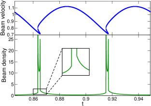
Figure 6: Beam density and beam velocity versus time for two periods from a Lagrangian TWT calculation accounting for space charge and circuit fields. The expanded view of the beam density is to highlight the density asymmetry about the peak.

Even though electrons experience forces due to space charge and circuit fields in a TWT, as can be inferred by comparing the beam velocities of Figs. 5 and 6, the cause of phase distortion is the same. Electrons slowed down from the dc beam velocity will spread more in time than electrons sped up from the dc beam velocity. The result is that the density wave form has a relatively higher density behind the peak than in front of it, as seen in Fig. 6.

In Refs. [3, 4] we described phase distortion from a frequency domain perspective as a “self-intermodulation” process, whereby harmonic distortions mix with the fundamental to produce distortions at the fundamental. Below we outline this view of phase distortion so that it may be compared to the time domain view given above.

If we express the velocity $u$ and density $\rho$ with Fourier series (for periodic inputs), then the fundamental frequency components of nonlinear products of $\rho$ and $u$ are seen to come from mixing of the second harmonic with the fundamental frequency, and mixing of higher order harmonics. In particular, if we define state variable envelopes as in Refs. [3, 4], e.g.,

$$u(x,t) = \sum_{m=-\infty}^{\infty}{\hat{u}_{m}}(x)e^{im\omega(x-t)},$$ (19)

then the continuity equation for the force-free drifting beam gives

$$\frac{d{\hat{\rho}_{\ell}}}{dx} = -i\ell\omega{\hat{u}_{n}}+i\sum_{m,n\neq 0\atop m+n=\ell}m\omega{\hat{u}_{m}}{\hat{u}_{n}}$$ (20)

$$\mbox{}-i\ell\omega\sum_{m,n\neq 0\atop m+n=\ell}{\hat{u}_{m}}{\hat{\rho}_{n}}$$

where the approximations used in Refs. [3, 4] have been made. From Eq. (20) products of frequencies such as $(m,n)=(-1,2),(2,-1),(-2,3),(3,-2),$ etc. are seen to influence the fundamental frequency $\ell=1$. In Refs. [3, 4] we considered $(m,n)=(-1,2),(2,-1)$ (third order intermodulation, “$3\,$IM”) and $(m,n)=(-2,3),(3,-2)$ ($5\,$IM) contributions to phase distortion in linear beam devices.

Equation (20) together with the corresponding nonlinear envelope equation for the velocity has an analytic solution that may be expressed in an infinite series of complex exponentials. The first terms in the series correspond to the linear solution as seen in Fig. 1. The linear terms are used in the equation for the second harmonic envelopes to produce the first terms in the series solution at the second harmonic. The second harmonic terms are then combined with the linear terms from the fundamental solution to produce the next set of terms at the fundamental. These complex exponentials add to the linear density solution and produce a phase shift (distortion) in the density solution. As it turns out, this process of generating harmonics and then additional terms at the fundamental must be continued to get an accurate representation of the nonlinear phase shifted density seen in Fig. 1. For the example in Fig. 1 we found that terms higher than $11\,$IM were required to adequately approximate the nonlinear density, whereas in Refs. [3, 4] we found that $5\,$IMs were sufficient to predict the phase distortion. The difference between the two cases is that the case in Fig. 1 has a much larger relative input modulation.

We have identified the mechanism for phase distortion in the simplest system that pertains to linear beam vacuum devices, the force-free drifting electron beam. The dominant cause of phase distortion is shown to be the inverse dependence of arrival time for an electron on its velocity, i.e., the “$1/u$ nonlinearity,” and that a secondary cause of phase distortion is the nonlinearity of the velocity modulation. Although we show this to be the case for the force-free drifting beam, we claim that the $1/u$ nonlinearity is also the cause of phase distortion in other linear beam devices, such as the traveling wave tube. That is, even though electrons are experiencing forces from the circuit and space charge fields, the fact remains that charges slowed down from the dc beam velocity will stretch and compress more than charges sped up from the dc beam velocity. Results from a traveling wave tube calculation are given that show the same characteristic asymmetric density modulation that is seen in the force-free drifting beam. We also show that the $1/u$ nonlinearity is the cause of phase distortion regardless of whether drive levels are strong enough such that electron overtaking occurs.

The identification of the mechanism for phase distortion suggests how inputs might be tailored to ameliorate phase distortion. The obvious candidates would involve somehow reducing the amplitude of the velocity modulation on the negative half cycle to lessen the effect of the “enhanced stretching,” or to provide a density modulation $180^{\circ}$ out of phase from the velocity modulation so that the “enhanced stretching” before the peak starts from a higher density value relative to the density behind the peak, and would be balanced about the density peak at the output. The latter scheme may be facilitated by cold cathode technology [2]. It is anticipated that either of these schemes, and potentially any scheme, may come with an associated gain compression, as in Ref. [3] where harmonic injection was used to set the fundamental output phase at a cost of reducing output power. It is also possible that further study may show that any tailoring of the velocity modulation may just be a manifestation of harmonic injection, proving the usefulness of the complementary views of phase distortion given in this note and in Refs. [3, 4].

References

- [1] Y.Y. Lau, D.P. Chernin, C. Wilsen, and R.M. Gilgenbach. Theory of intermodulation in a klystron. IEEE Trans. Plasma Sci., 28(3):959–970, June 2000.
- [2] D.R. Whaley, B.M. Gannon, V.O. Heinen, K.E. Kreischer, C.E. Holland, and C.A. Spindt. Experimental demonstration of an emission-gated traveling-wave tube amplifier. IEEE Trans. Plasma Sci., 30(3):998–1008, June 2002.
- [3] J.G. Wöhlbier and J.H. Booske. Mechanisms for phase distortion in a traveling wave tube. Phys. Rev. E, 69, 2004. 066502.
- [4] J.G. Wöhlbier and J.H. Booske. Nonlinear space charge wave theory of distortion in a klystron. IEEE Trans. Electron Devices, 2005. To appear.
- [5] J.G. Wöhlbier, J.H. Booske, and I. Dobson. The Multifrequency Spectral Eulerian (MUSE) model of a traveling wave tube. IEEE Trans. Plasma Sci., 30(3):1063–1075, 2002.
- [6] J.G. Wöhlbier, S. Jin, and S. Sengele. Eulerian calculations of wave breaking and multi-valued solutions in a traveling wave tube. Phys. Plasmas, 2005. To appear.