Bijectivity of the Normalization and Fermi-Coulomb Hole Sum Rules for Approximate Wave Functions

Abstract

We prove the bijectivity of the constraints of normalization and of the Fermi-Coulomb hole charge sum rule at each electron position for approximate wave functions. This bijectivity is surprising in light of the fact that normalization depends upon the probability of finding an electron at some position, whereas the Fermi-Coulomb hole sum rule depends on the probability of two electrons staying apart because of correlations due to the Pauli exclusion principle and Coulomb repulsion. We further demonstrate the bijectivity of these sum rules by example.

Sum rules play an important role in physics, and there are many ways in which they are employed. Within the realm of electronic structure theory, for example, accurate properties of a system may be determined by the use of an approximate potential whose parameters are adjusted so as to ensure the satisfaction of a sum rule. Metal surface properties such as the surface energy and work function are obtained by application of the Theophilou-Budd-Vannimenus sum rule 1 which relates the value of the electrostatic potential at the surface to the known bulk properties of the metal. The parameters in a model effective potential at a metal surface are then adjusted 2 so as to satisfy this sum rule. Another manner in which sum rules have proved to be significant is in the context of Kohn-Sham density functional theory (KS-DFT) 3 , a local effective potential theory of electronic structure that is extensively employed in atomic, molecular, and condensed matter physics. In KS-DFT, all the many-body effects are incorporated in the ‘exchange-correlation’ energy functional of the ground state density. Since this functional is unknown, it must be approximated. A successful approach 4 to the construction of approximate ‘exchange-correlation’ energy functionals, and of their derivatives which represent the local effective potential in the theory, is the requirement of satisfaction of various scaling laws 5 together with those of sum rules on the Fermi and Coulomb hole charge distributions 6 . In the recently developed Quantal density functional theory (Q-DFT) 6 , the local effective potential is described instead in terms of the system wave function. Thus, one method for the construction of the local effective potential in Q-DFT is to employ an approximate wave function that is a functional of some functions 7 . These latter functions are determined such that the wave function functional satisfies various constraints such as normalization, the Fermi-Coulomb or Coulomb hole sum rules, or reproduces a physical observable of interest such as the density, diamagnetic susceptibility, nuclear magnetic constant, etc.7 .

The satisfaction of a particular sum rule by an approximate potential, or an ‘exchange-correlation’ energy functional, or a wave function functional, however, does not necessarily imply the satisfaction of other sum rules. In this paper we describe a counter intuitive bijective relationship between the sum rules of normalization and that of the Fermi-Coulomb or Coulomb hole charge. The satisfaction of either one of the sum rules by an approximate wave function ensures the satisfaction of the other. This bijectivity is counter intuitive because the constraints of normalization and of the Fermi-Coulomb hole depend on distinctly different quantum-mechanical probabilities. The bijectivity is also of importance from a practical numerical perspective. The proof and demonstration of the bijectivity of these sum rules constitutes the paper.

To understand why this bijectivity is so counter to intuition, let us consider the physics underlying the two properties of an electronic system that these sum rules depend upon. For a system of $N$ electrons, the constraint of normalization on an approximate wave function $\Psi({\bf X})$ requires that

$$\int\Psi({\bf X})^{*}\Psi({\bf X})d{\bf X}=1,$$ (1)

where ${\bf X}={\bf x}_{1},...,{\bf x}_{N};d{\bf X}=d{\bf x}_{1},...,d{\bf x}_{N};{\bf x}={\bf r},s$ with ${\bf r}$ and $s$ being the spatial and spin coordinates of an electron. (Atomic units $e=\hbar=m=1$ are assumed.) Equivalently, this sum rule may be written in terms of the electronic density $\rho({\bf r})$. The density $\rho({\bf r})$ is $N$ times the probability of an electron being at ${\bf r}$ :

$$\rho({\bf r})=N\sum_{i}\int\Psi^{*}({\bf r}\sigma,{\bf X}^{N-1})\Psi({\bf r}\sigma,{\bf X}^{N-1})d{\bf X}^{N-1},$$ (2)

where $d{\bf X}^{N-1}=d{\bf x}_{2},...,d{\bf x}_{N}$. The normalization sum rule then becomes

$$\int\rho({\bf r})d{\bf r}=N.$$ (3)

The density $\rho({\bf r})$ is a static or local charge distribution. By this is meant that its structure remains unchanged as a function of electron position ${\bf r}$. Integration of this charge distribution—the normalization sum rule—then gives the number $N$ of electrons. Thus, normalization is a statement as to the number of electrons in the system.

The definition of the Fermi-Coulomb hole charge distribution $\rho_{xc}({\bf r}{\bf r}^{\prime})$ derives from that of the pair-correlation density $g({\bf r}{\bf r}^{\prime})$. The pair-correlation density is the density at ${\bf r}^{\prime}$ for an electron at ${\bf r}$. The density at ${\bf r}^{\prime}$ differs from that at ${\bf r}$ because of electron correlations due to the Pauli exclusion principle and Coulomb repulsion. Thus, the pair density is defined as

$$g({\bf r}{\bf r}^{\prime})=\langle\Psi|\sum_{i\neq j}\delta({\bf r}_{i}-{\bf r})\delta({\bf r}_{j}-{\bf r}^{\prime})|\Psi\rangle/\rho({\bf r}).$$ (4)

Its total charge, for each electron position ${\bf r}$, is therefore

$$\int g({\bf r}{\bf r}^{\prime})d{\bf r}^{\prime}=N-1.$$ (5)

The pair-correlation density $g({\bf r}{\bf r}^{\prime})$ is a dynamic or nonlocal charge distribution in that its structure changes as a function of electron position for nonuniform electron density systems. If there were no electron correlations, the density at ${\bf r}^{\prime}$ would be $\rho({\bf r}^{\prime})$. Hence, the pair-correlation density is the density at ${\bf r}^{\prime}$ plus the reduction in density at ${\bf r}^{\prime}$ due to the electron correlations. The reduction in density about an electron which occurs as a result of the Pauli exclusion principle and Coulomb repulsion is the Fermi-Coulomb hole charge $\rho_{xc}({\bf r}{\bf r}^{\prime})$. Thus, the Fermi-Coulomb hole is defined as

$$\rho_{xc}({\bf r}{\bf r}^{\prime})=g({\bf r}{\bf r}^{\prime})-\rho({\bf r}^{\prime}).$$ (6)

The Fermi-Coulomb hole $\rho_{xc}({\bf r}{\bf r}^{\prime})$ about an electron is also a dynamic or nonlocal charge distribution. For nonuniform electron gas systems, its structure is different for each electron position. Since each electron digs a hole in the inhomogeneous sea of electrons equal in charge to that of a proton, it follows that the total charge of the Fermi-Coulomb hole surrounding an electron, for each electron position ${\bf r}$, is

$$\int\rho_{xc}({\bf r}{\bf r}^{\prime})d{\bf r}^{\prime}=-1.$$ (7)

This is the Fermi-Coulomb hole sum rule.

The definition of the Coulomb hole $\rho_{c}({\bf r}{\bf r}^{\prime})$, which is the reduction in density at ${\bf r^{\prime}}$ for an electron at ${\bf r^{\prime}}$ because of Coulomb repulsion, in turn derives from that of the Fermi-Coulomb $\rho_{xc}({\bf r}{\bf r}^{\prime})$ and Fermi $\rho_{x}({\bf r}{\bf r}^{\prime})$ holes. The Fermi hole is the reduction in density at ${\bf r^{\prime}}$ for an electron at ${\bf r}$ that occurs due to the Pauli exclusion principle. The Fermi hole is defined via the pair-correlation density $g_{s}({\bf r}{\bf r}^{\prime})$ derived through a normalized Slater determinant $\Phi\{\varphi_{i}\}$ of single particle orbitals $\varphi_{i}({\bf x})$:

$$g_{s}({\bf r}{\bf r}^{\prime}) = \frac{\langle\Phi\{\varphi_{i}\}|\sum_{i\neq j}\delta({\bf r}_{i}-{\bf r})\delta({\bf r}_{j}-{\bf r}^{\prime})|\Phi\{\varphi_{i}\}\rangle}{\rho({\bf r})}$$ (8)

$$= \rho({\bf r}^{\prime})+\rho_{x}({\bf r}{\bf r}^{\prime}).$$ (9)

The orbitals $\varphi_{i}({\bf x})$ may be generated either through KS-DFT or Q-DFT in which case the density $\rho({\bf r})$ is the same as that of the interacting system, or they could be the Hartree-Fock theory orbitals for which the density is different. As the sum rule on $g_{s}({\bf r}{\bf r}^{\prime})$ is the same as in Eq. (5), and the Slater determinant is normalized, the total charge of the Fermi hole, for each electron position ${\bf r}$, is also that of a proton:

$$\int\rho_{x}({\bf r},{\bf r}^{\prime})d{\bf r}^{\prime}=-1.$$ (10)

The Coulomb hole is then defined as the difference between the Fermi-Coulomb and Fermi holes:

$$\rho_{c}({\bf r}{\bf r}^{\prime})=\rho_{xc}({\bf r}{\bf r}^{\prime})-\rho_{x}({\bf r}{\bf r}^{\prime}).$$ (11)

. The total charge of the Coulomb hole, for each electron position ${\bf r}$, is therefore zero:

$$\int\rho_{c}({\bf r}{\bf r}^{\prime})d{\bf r}^{\prime}=0.$$ (12)

This is the Coulomb hole sum rule.

Both the normalization and the Fermi-Coulomb or Coulomb hole constraints are charge conservation sum rules. However, their physical origin, and therefore the charge conserved in each case, is different. That these distinctly different charge conservation rules are intrinsically linked bijectively constitutes the theorem we prove.

Theorem: The normalization and Fermi-Coulomb or Coulomb hole sum rules are bijective. Satisfaction of the normalization sum rule by an approximate wave function implies the automatic satisfaction of the Fermi-Coulomb or Coulomb hole sum rules for each electron position. Conversely, the satisfaction of the Fermi-Coulomb or Coulomb hole sum rules for each electron position by an approximate wave function implies the normalization of that wave function:

$$\left(\begin{array}[]{c}\int\Psi({\bf X})^{*}\Psi({\bf X})d{\bf X}=1\\ or\\ \int\rho({\bf r})d{\bf r}=N\end{array}\right)\begin{array}[]{c}\rightarrow\\ \leftarrow\end{array}\left(\begin{array}[]{c}\int\rho_{xc}({\bf r}{\bf r}^{\prime})d{\bf r}^{\prime}=-1\\ or\\ \int\rho_{c}({\bf r}{\bf r}^{\prime})d{\bf r}^{\prime}=0\end{array}\right)$$ (13)

Proof: (a)The proof of the arrow to the right in Eq. (13) is as follows. Let us assume an approximate wave function that is normalized. Then, integration of Eq.(6) over ${\bf r}^{\prime}$ using the normalization constraint of Eq.(3) leads directly to the Fermi-Coulomb hole sum rule of Eq.(7).
(b) For the arrow to the left, consider an approximate wave function that satisfies the Fermi-Coulomb hole sum rule Eq.(7) for each electron position ${\bf r}$. The sum rule Eq.(5) on the pair-correlation density $g({\bf r}{\bf r}^{\prime})$ follows from its definition Eq.(4) which is independent of whether or not the wave function is normalized. Thus, since both the sum rules on the Fermi-Coulomb hole and the pair-correlation density are satisfied, then on integration of Eq.(6) over ${\bf r}^{\prime}$, normalization of the wave function is ensured.
(c) Consider an approximate wave function from which one constructs a Fermi-Coulomb hole for each electron position ${\bf r}$. For a normalizd Slater determinant $\Phi\{\varphi_{i}\}$, next define a Fermi hole $\rho_{x}({\bf r}{\bf r}^{\prime})$ which then satisfies the Fermi hole sum rule of Eq.(10). If the satisfaction of the Coulomb hole sum rule is now ensured, then this guarantees the satisfaction of the Fermi-Coulomb hole sum rule, which as shown in (b), ensures that the wave function is normalized.

Recall that normalization depends upon the probability of finding an electron at some position. On the other hand, the Fermi-Coulomb and Coulomb hole sum rules depend on the reduction in probability of two electrons approaching each other. The fact that satisfaction of the integral condition of either one of these probabilities means the satisfaction on the integral condition of the other is not obvious, and therefore surprising.

We next demonstrate the bijectivity of Eq. (13) by application to the ground state of the Helium atom. The nonrelativistic Hamiltonian of the atom is

$$\hat{H}=-\frac{1}{2}\nabla_{1}^{2}-\frac{1}{2}\nabla_{2}^{2}-\frac{Z}{r_{1}}-\frac{Z}{r_{2}}+\frac{1}{r_{12}},$$ (14)

where ${\bf r}_{1}$, ${\bf r}_{2}$ are the coordinates of the two electrons, $r_{12}$ is the distance between them, and $Z=2$ is the atomic number. The equivalence from left to right of Eq. (13) can be easily demonstrated by assuming an approximate wave function $\psi$ with parameters $c_{i}(i=1,...,p)$ that is normalized in the standard manner at the energy minimized values of the parameters: $\frac{\partial I[\psi]}{\partial c_{i}}=0$, where $I[\psi]=\int\psi^{*}H\psi d\tau/\int\psi^{*}\psi d\tau$. On the other hand, the equivalence from right to left is not as readily accomplished through such a wave function since the Fermi-Coulomb hole sum rule must be satisfied at each electron position. It is, however, possible to demonstrate the bijectivity by assuming the wave function to be a functional of a set of functions $\chi$: $\psi=\psi[\chi]$ instead of simply a function. The functions $\chi$ are determined so as to satisfy the normalization or Fermi-Coulomb hole sum rules as described in Ref.7.

Table 1: The satisfaction of the Coulomb hole sum rule Eq.(12) for different electron positions ${\bf r}$ 9 .

${\bf r}$(a.u.)	$\;\;\;\;\;\int\rho_{c}({\bf r}{\bf r}^{\prime})d{\bf r}^{\prime}\;\;\;\;$
0.00566798	-0.00039251
0.13567807	0.00032610
0.57016010	0.00034060
0.72285115	0.00013025
0.89208965	0.00001584
1.07722084	0.00007529
1.49223766	0.00029097
1.96148536	0.00034743
3.91996382	0.00032567
5.15549169	0.00057862

For the left to right equivalence, we choose the wave function functional to be of the form 7

$$\psi[\chi]=\Phi(\alpha,s)[1-f(\chi;s,u)],$$ (15)

with$\Phi[\alpha,s]=(\alpha^{3}/\pi)e^{-\alpha s}$, $f(s,u)=e^{-qu}(1+qu)[1-\chi(q;s,u)(1+u/2)]$, where $\alpha$ and $q$ are variational parameters, $s=r_{1}+r_{2},u=r_{12}$. The function $\chi=\chi_{2}$ of 7 , with the energy minimized values of the parameters being $\alpha=1.6629,q=0.17049$. This wave function is normalized to unity, the function $\chi$ being determined as a solution to a quadratic equation. We further assume, as in local effective potential energy theory, that the Fermi hole $\rho_{x}({\bf r}{\bf r^{\prime}})=-\rho({\bf r^{\prime}})/2$. The corresponding Coulomb holes $\rho_{c}({\bf r}{\bf r^{\prime}})$ are plotted in Figs. $1$ and $2$ for electron positions at ${r}=0,0.566,0.8,1.0$ (a.u.) together with the exact Coulomb hole 8 . (The electron is on the $z$ axis corresponding to $\theta=0$. The cross section through the Coulomb hole plotted corresponds to $\theta^{\prime}=0$ with respect to the electron-nucleus direction. The graph for $r^{\prime}<0$ corresponds to the structure for $\theta^{\prime}=\pi$ and ${r}^{\prime}>0$.) The two Coulomb holes, though similar are inequivalent. Integration of both the exact and approximate Coulomb holes for each electron position leads to a total charge of zero.

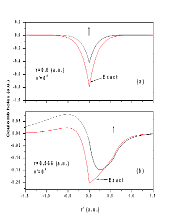
Figure 1: Cross-section through the Coulomb holes for electron positions at (a)$r=0$ (a.u.), and (b) $r=0.566$ (a.u.). The holes determined by the wave function functional of Eq.(15) and the ‘exact’ hole are plotted .

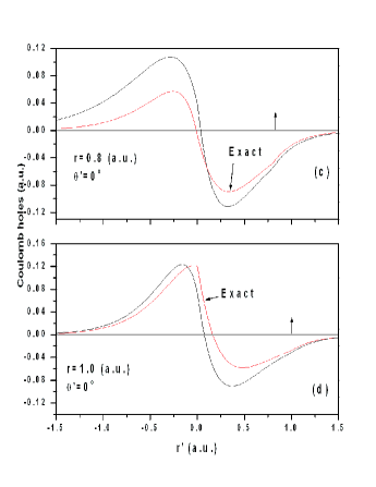
Figure 2: The figure caption is the same as in Fig.1 except that the cross sections plotted are for electron positions at (c)$r=0.8$ (a.u.), and (d) $r=1.0$ (a.u.). .

For the right to left equivalence of Eq. (13), we choose a different wave function functional 9 :

$$\psi[\chi]=\Phi(\phi_{i})[1-f({\bf r}_{1}{\bf r}_{2})],$$ (16)

with $f({\bf r}_{1}{\bf r}_{2})=e^{-\beta^{2}r^{2}}[1-\chi({\bf R})(1+r/2))]$ , ${\bf r}={\bf r}_{1}-{\bf r}_{2}$, ${\bf R}=({\bf r}_{1}+{\bf r}_{2})/2$, $\beta=q[\rho({\bf R})]^{1/3}$, $q$ a variational parameter, and $\Phi(\phi_{i})$ the Hartree-Fock theory prefactor 10 . The satisfaction of the Coulomb hole sum rule requires the solution of a nonlinear integral Fredholm equation of the first kind for the determination of the function $\chi({\bf R})$. We have solved 9 the linearized version of this integral equation for $\chi({\bf R})$. The satisfaction of the Coulomb hole sum rule for typical electron positions for $q=1$ is given in Table I. (We do not plot the corresponding Coulomb holes as they are very similar to those of Figs. 1 and 2.) The wave function functional of Eq. (16) thus determined satisfies the normalization constraint to the same degree of accuracy as that of the sum rule given in Table I. Hence, the bijectivity of the normalization and Coulomb hole sum rules is demonstrated by example.

In conclusion, we have proved the bijectivity of the normalization and Fermi-Coulomb or Coulomb hole sum rules for approximate wave functions. The bijectivity is also significant from a numerical perspective because it is much easier to normalize a wave function than to ensure the satisfaction of the Fermi-Coulomb or Coulomb hole sum rules for each electron position. As shown by the examples, the determination of a wave function functional via normalization requires the solution of a quadratic equation, whereas that determined via satisfaction of the Coulomb hole sum rule requires the solution of an integral equation. On the other hand we note that the wave function functionals, as determined by satisfaction of the different sum rules, are different. Hence, the Fermi-Coulomb and Coulomb holes, and therefore how the electrons are correlated, will be different depending upon which sum rule is satisfied. It is unclear as to whether a better representation of the electron correlations is achieved by satisfaction of the normalization sum rule or that of the Fermi-Coulomb hole. Finally, the bijectivity explains the results of our analysis 11 of the Colle-Salvetti wave function functional 12 . This wave function, which constitutes the basis for the most extensively used correlation energy functional in the literature, is of the same form as that of Eq. (16) except that $\chi({\bf R})=\sqrt{\pi}\beta/(1+\sqrt{\pi}\beta)$, $\beta=q[\rho^{HF}({\bf R})]^{1/3}$. In analyzing this wave function we had noted that it was neither normalized nor did it satisfy the Coulomb hole sum rule. These facts are consistent with the bijectivity theorem proved above. The lack of satisfaction of either one of the constraints ensures the lack of satisfaction of the other.

- (1) A. K. Theophilou, J. Phys. F 2, 1124 (1972); H. F. Budd and J. Vannimenus, Phys. Rev. Lett. 31, 1218 (1973); 31, 1430 (E) (1973); J. Vannimenus and H. F. Budd, Solid State Commun. 15, 1739 (1974).
- (2) V. Sahni, C. Q. Ma, and J. Flamholz, Phys. Rev. B 18, 3931 (1978).
- (3) W. Kohn and L. J. Sham, Phys. Rev. 140, A1133 (1965).
- (4) J. P. Perdew, J. Chem. Phys. (to appear); J. P. Perdew, Phys. Rev. Lett. 55, 1665 (1985).
- (5) M. Levy, Adv. Quantum Chem. 21, 69 (1990); S. Ivanov and M. Levy, Adv. Quantum Chem. 33, 11 (1998).
- (6) V. Sahni, Quantal Density Functional Theory, (Springer-Verlag, berlin, 2004).
- (7) X.-Y. Pan, V. Sahni. and L. Massa, Phys. Rev. Lett. 93, 130401 (2004).
- (8) M. Slamet and V. Sahni, Phys. Rev. A 51, 2815 (1995).
- (9) R. Singh, V. Sahni, and L. Massa (manuscript in preparation).
- (10) E. Clementi and C. Roetti, Atom. Data Nucl. Data Tables 14, 177 (1974).
- (11) R. Singh, L. Massa, and V. Sahni, Phys. Rev A 60, 4135 (1999).
- (12) R. Colle and O. Salvetti, Theor. Chim. Acta 37, 329 (1975).