Interface effects and termination of finite length nanotubes

Abstract

The objective of the present paper is to investigate interface effects in carbon nanotubes. We use both real and k-space tight binding method. We study in detail the effect of wrapping vector on the electronic properties. We analyze the effect of the curvature in closed nanotube to the electronic properties. The finite length of the nanotube affects the electronic properties.

I Introduction

A carbon nanotube is obtained when the honeycomb graphene sheet is wrapped into a seamless cylinder iijima . The electronic properties are sensitive on its geometrical structure. Depending on the orientation of the hexagons with respect to the nanotube axis, they can be classified to ’armchair’, ’zigzag’, and ’chiral’. The single wall nanotubes (SWNT), which consist of a single graphite layer, have diameter around $1-2$nm and they are proposed as ideal components for the future nano devices.

Scanning tunneling microscopy and spectroscopy on individual SWNT has been used recently to provide atomically resolved images and to allow the determination of the nanotube electronic properties as a function of the wrapping vector and diameter wildoer .

The electronic properties of hybrid structures of carbon nanotubes have already been analyzed theoretically within the Hubbard model (see in our previous work stefan3 ). We pointed out there that the finite length of nanotubes affects the properties of the hybrid structure.

In this paper we calculate within the real and $k$-space tight binding method the electronic properties of carbon nanotubes. We examine the effect of the chirality on the electronic properties. In addition we study termination of nanotubes i.e. the effect of the curvature at the cups of nanotube to the local density of states. We point out the differences between the two approaches. The real space method has the advantage that it permits the treatment of finite size samples.

In the following we describe the methods in Sec II. In Sec III we present the results using the k-space and real space tight binding method. We discuss the effect of chirality, and the termination of the nanotubes. In the last section we present the conclusions.

II method

II.1 k-space tight binding method

Tight binding theory in k-space has been used to calculate the electronic properties of nanotubes. The energy dispersion relation for nanotube is found from the two dimensional dispersion relation for the $\pi$ bands of graphite by eliminating one of the two components of the wave vector $k$ according to the periodic boundary conditions in the circumferential direction saito

$$C_{h}\dot{k}=2\pi m,$$ (1)

where $C_{h}=na_{1}+ma_{2}$ is the chiral vector, $a_{1},a_{2}$ are the unit cell basis vectors of graphite, and $n,m$ are integers. For example the energy dispersion relation for armchair nanotube is

$$E_{q}^{a}(k)=\pm t\{1\pm 4\cos(q\pi/n)\cos(ka/2)+4\cos^{2}(ka/2)\}^{1/2}.$$ (2)

For zig-zag nanotubes the corresponding dispersion relation reads

$$E_{q}^{z}(k)=\pm t\{1\pm 4\cos(q\pi/n)\cos(\sqrt{3}ka/2)+4\cos^{2}(q\pi/n)\}^{1/2}.$$ (3)

Using the one dimensional dispersion relations the density of states (DOS) is calculated using the following formulas economou

$$\rho(E)=\pm\frac{1}{\pi}im\{G(l,l;E)\},$$ (4)

where the diagonal matrix element of the Green function $G(l,l;z)$ in one dimension is

$$G(l,l;z)=\frac{1}{2\pi}\int_{-\pi}^{\pi}d\phi\frac{1}{z-E(\phi)}.$$ (5)

II.2 real space tight binding method

Within the second approach we describe the SWNT by exact diagonalizations of the real space tight binding Hamiltonian in a honeycomb latticestefan ; stefan1 ; stefan2 ; stefan3 . The corresponding Hamiltonian is written as

$$H=-t\sum_{<i,j>\sigma}c_{i\sigma}^{\dagger}c_{j\sigma}+\mu\sum_{i\sigma}n_{i\sigma},~{}~{}~{}$$ (6)

where $i,j$ are sites indices and the angle brackets indicate that the hopping is only to nearest neighbors, $n_{i\sigma}=c_{i\sigma}^{\dagger}c_{i\sigma}$ is the electron number operator in site $i$, $\mu$ is the chemical potential. Within tight binding method we solve the following eigenvalue problem

$$\hat{\xi}u_{n}(r_{i})=\epsilon_{n}u_{n}(r_{i}),~{}~{}~{}$$ (7)

where

$$\hat{\xi}u_{n}(r_{i})=-t\sum_{\hat{\delta}}u_{n}(r_{i}+\hat{\delta})+\mu u_{n}(r_{i}),~{}~{}~{}$$ (8)

and we obtain the eigenvectors $u(r_{i})$ and the eigenenergies $\epsilon_{n}$ self consistently. Then the local density of states (LDOS) at the $i$th site is calculated by

$$\rho_{i}(E)=-2\sum_{n}\left[|u_{n}(r_{i})|^{2}f^{{}^{\prime}}(E-\epsilon_{n})\right],~{}~{}~{}$$ (9)

where the factor $2$ comes from the twofold spin degeneracy, $f^{{}^{\prime}}$ is the derivative of the Fermi function,

$$f(\epsilon)=\frac{1}{\exp(\epsilon/k_{B}T)+1}.$$ (10)

For numerical stability reasons and in order to present more realistic results we set the temperature $T$ to a non zero value.

SWNT is formed by rolling the honeycomb sheet into a cylinder and using the appropriate boundary conditions to describe armchair and zigzag structures.

III results

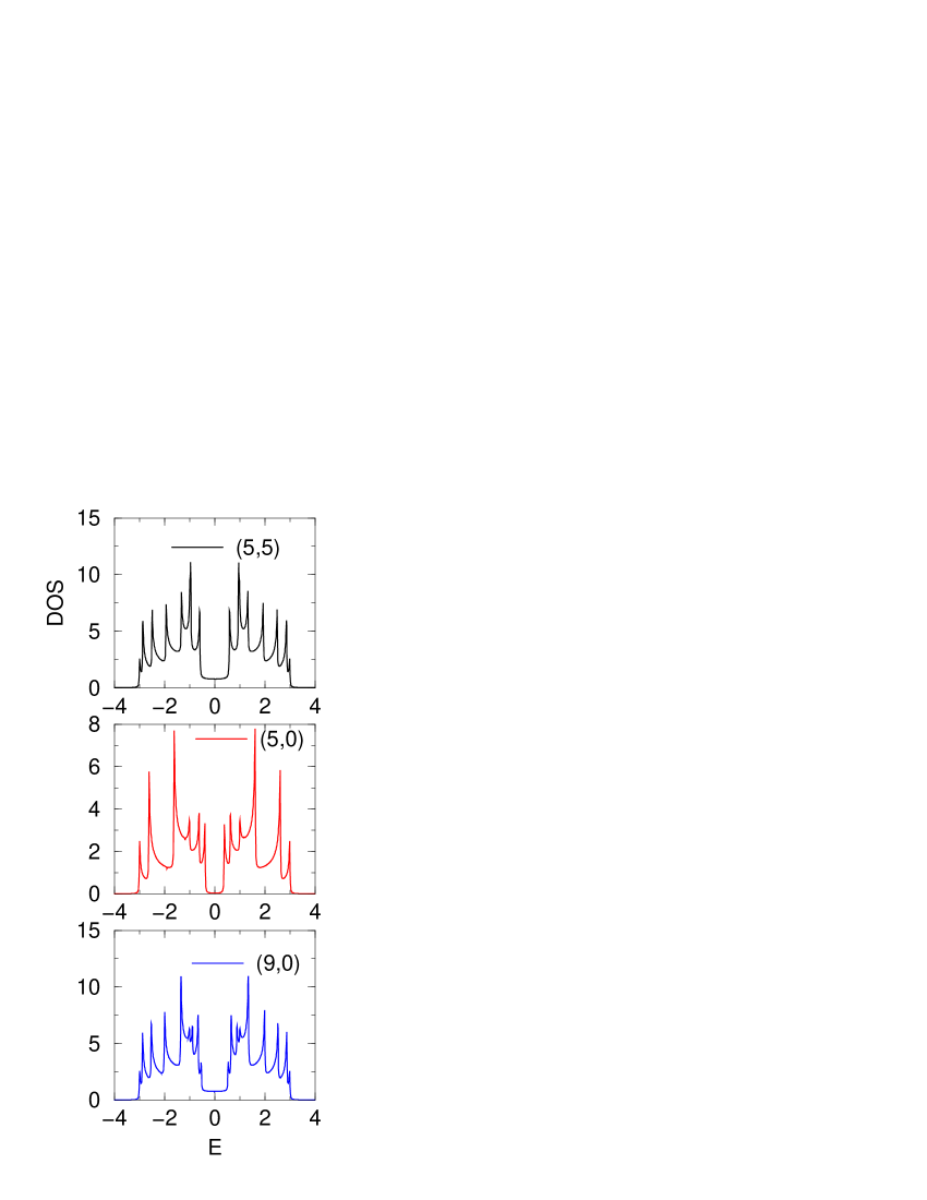
Figure 1: The DOS for several metallic and semiconducting nanotubes using the tight binding k-space approach.

We present first the well known results using the tight binding method in reciprocal space. We note that this method is restricted to description of nanotubes of infinite length. In Fig. 1 we show the DOS for several nanotube structures. In order to analyze the density of states we have to take into account the dispersion relation of nanotubes. The dispersion relation of nanotube consists of $2n$ curves for the valence and conduction bands respectively. For armchair nanotube the valence and conduction bands cross at the Fermi level. Therefore the armchair nanotube is metallic as indicated by the finite density of states at $E=0$ in Fig. 1. We also observe singularities at the band edges which correspond to the extrema of $E(k)$ relations. For zig-zag nanotube ($n,0$) when $n$ is not multiply of $3$ the dispersion relation curves do not cross at the Fermi level. As a consequence the nanotube is semiconducting with an energy gap at the Fermi energy as seen in Fig. 1 for the ($5,0$) nanotube. An exception occurs when $n$ is a multiply of $3$. For example in the $(9,0)$ nanotube which is shown at the bottom of the figure, we note that although its geometry corresponds to a zig-zag nanotube, it is actually metallic since analysis of the energy dispersion relation shows that the valence and conduction bands cross each other at the Fermi level at the $\Gamma$ point ($k=0$).

We present now the results for the real space tight binding method. Contrary to the previous case which is restricted to infinite length nanotubes, this approach permits the description of structures that are of finite length. Since the modern nanodevices require finite length components this approach is more advanced compared to the $k$ space approach. The LDOS close to the boundary for the two dimensional graphite lattice which is presented in Fig. 2 shows strong deviation from the bulk value (see Fig. 3). It is well known that the bulk graphite is zero gap semiconductor which is not the case for graphene nanosamples close to the interface since there are curves with finite DOS at the Fermi level. We study then the armchair $(5,5)$ nanotube seen in Fig. 4. The LDOS shown in Fig. 5 shows finite states in the Fermi level which indicate that the SWNT is metallic. This agrees with the previous $k$-space approach. However we find that the LDOS is strongly modulated close to the boundary (see sites A,B,C in Fig. 5) from the bulk D site. Even-more at specific sites e.g. C the LDOS approaches zero which indicates insulating behavior. An other characteristic is the presence of bands with one-dimensional Van-Hove singularities at the band edges. Due to the finite temperature that we use the overall line shape is smooth.

We would like to describe other nanotubes like the zig-zag which is shown in Fig. 6. This nanotube is expected to be semiconducting. We confirm that for the bulk. However close to the surface a peak appears at specific sites (see Fig. 7). This is opposite to the $k$-space method.

We also describe the chiral nanotube which is shown in Fig. 8. This nanotube is semiconducting since $n-m$ is not a multiply of $3$. The magnitude of the semiconducting gap depends on the chiral vector and is different than the other semiconducting structures that we studied e.g. $(5,0)$. However close to the surface a peak appears at specific sites (see Fig. 9).

We discuss the termination of nanotubes. We specifically show that a geometrical and topological effect like the introduction of pentagons in a hexagonal lattice affects not only the curvature of the nanotube but also its electronic properties. We show in Fig. 10 the termination of an armchair nanotube using a cup which consists of a hemisphere of a fullerene. The cup contains six pentagons and an appropriate number of hexagons. The LDOS close to the end of the nanotube is deviating from the metallic behavior as seen in Fig. 11. As we can observe a peak is developing close to Fermi energy which corresponds to localized states that are formed due to the deformation of the lattice by the introduction of the pentagons. In order to investigate the effect of the cup to the nanotube we study then the electronic structure of the isolated nanocone. This is formed by placing six pentagons and appropriate number of hexagons such as a cone structure is formed (see in Fig. 12). This cone nanostructure closes exactly the $(5,5)$ nanotube and constitutes a half fullerene molecule. As is seen the bound states still exist. However due to the drastic reduction of the number of atoms the produced nanostructure has density of states which resembles that of a molecule with discrete bound levels (see Fig. 13).

Using the same procedure is possible to terminate a zig-zag nanotube. We show in Fig. 14 the termination of a zig-zag nanotube using appropriate number of pentagons. The LDOS close to the end of the nanotube is seen in Fig. 15. Here the peak which corresponds to the localized states around the pentagons exists at the Fermi energy. In order to investigate the effect of the cup to the $(5,0)$ nanotube we study then the electronic structure of the isolated nanocone. This is formed by placing six pentagons and appropriate number of hexagons such as a cone structure is formed (see in Fig. 16). This cone nanostructure closes exactly the $(5,0)$ nanotube. As is seen the bound states still exist. However due to the drastic reduction of the number of atoms the produced nanostructure has density of states which resembles that of a molecule with discrete bound levels (see Fig. 17).

IV conclusions

We have studied the electronic properties of finite length SWNT with in the tight binding method self consistently. This method provides advantages compared to the $k$-space method, namely that it permits the study of finite length nanotubes, which are expected to become the building blocks of the future nanodevices. The results indicate that for finite length nanotubes the LDOS is strongly modified close to the boundary layers of the nanotube. Moreover the local density of states changes considerably around the pentagons that terminate a nanotube where additional bound states are formed.

We have to make a distinction between the topological defects which we have studied in the present work and which do affect the electronic and transport properties of nanotubes and the mechanical deformations which result from bending twisting, and compressing the nanotube. The later in the absence of topological defects have minor effect to the electronic properties.

When studying the electronic properties of nanotubes the $sp^{2}$ hybridization of the atomic orbitals which has been used here, produces realistic results provided that the diameter of the nanotube is large enough. Concerning purely mechanical properties the $sp^{3}$ hybridization would produce more realistic results.

V acknowledgments

This work was supported in part from a stipend from ULB.

Figure 2: The graphite lattice close to the corner.

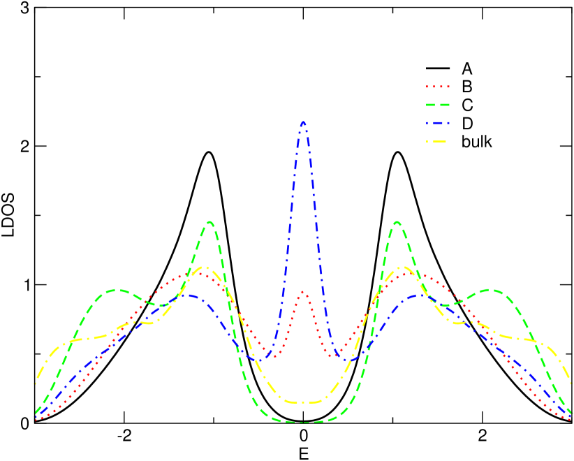
Figure 3: The LDOS for points A,B,C,D seen in Fig. 2 and the bulk LDOS.

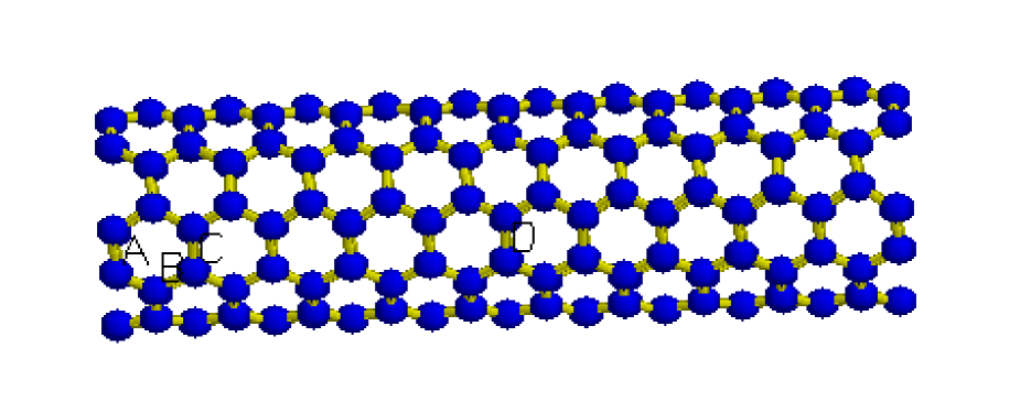
Figure 4: The open armchair $(5,5)$ nanotube composed of 21 layers.

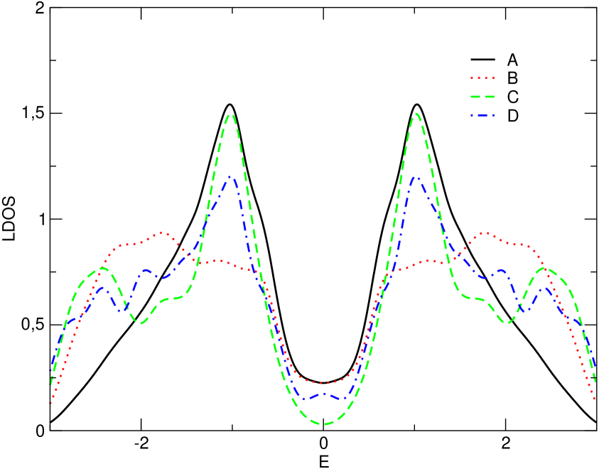
Figure 5: The LDOS for points A,B,C,D of the armchair $(5,5)$ nanotube seen in Fig. 4.

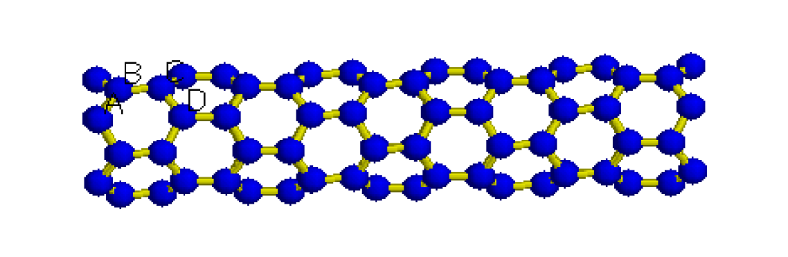
Figure 6: The open zigzag $(5,0)$ nanotube composed of 20 layers.

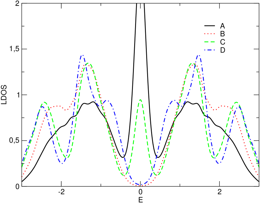
Figure 7: The LDOS for points A,B,C,D of a zig-zag $(5,0)$ nanotube.

Figure 8: The open chiral $(4,2)$ nanotube.

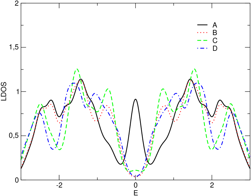
Figure 9: The LDOS for points A,B,C,D of a chiral $(4,2)$ nanotube.

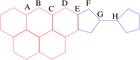
Figure 10: The closing of an armchair $(5,5)$ nanotube.

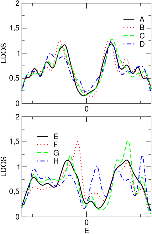
Figure 11: The LDOS for the points A,B,C,D,E,F,G,H that are seen in the previous figure closing the end of an armchair $(5,5)$ nanotube.

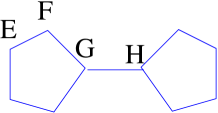
Figure 12: The geometry of a $(5,5)$ nanocone.

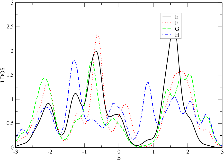
Figure 13: The LDOS for the points E,F,G,H that are seen in the figure 12 at the $(5,5)$ nanocone.

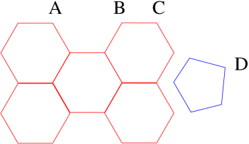
Figure 14: The closing of a zig-zag $(5,0)$ nanotube.

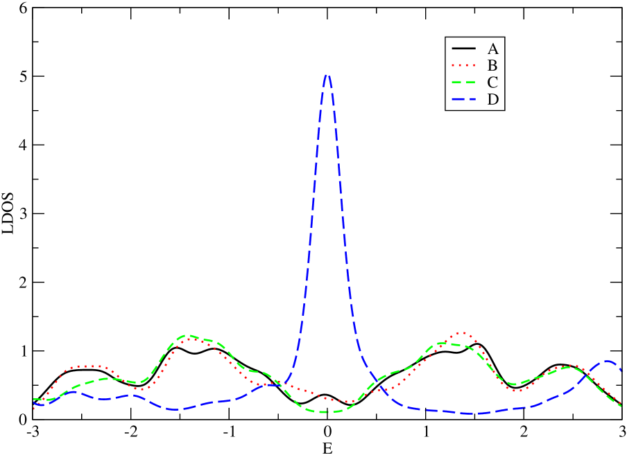
Figure 15: The LDOS for the points A,B,C,D that are seen in the previous figure closing the end of a zig-zag $(5,0)$ nanotube.

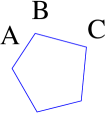
Figure 16: The geometry of a $(5,0)$ nanocone.

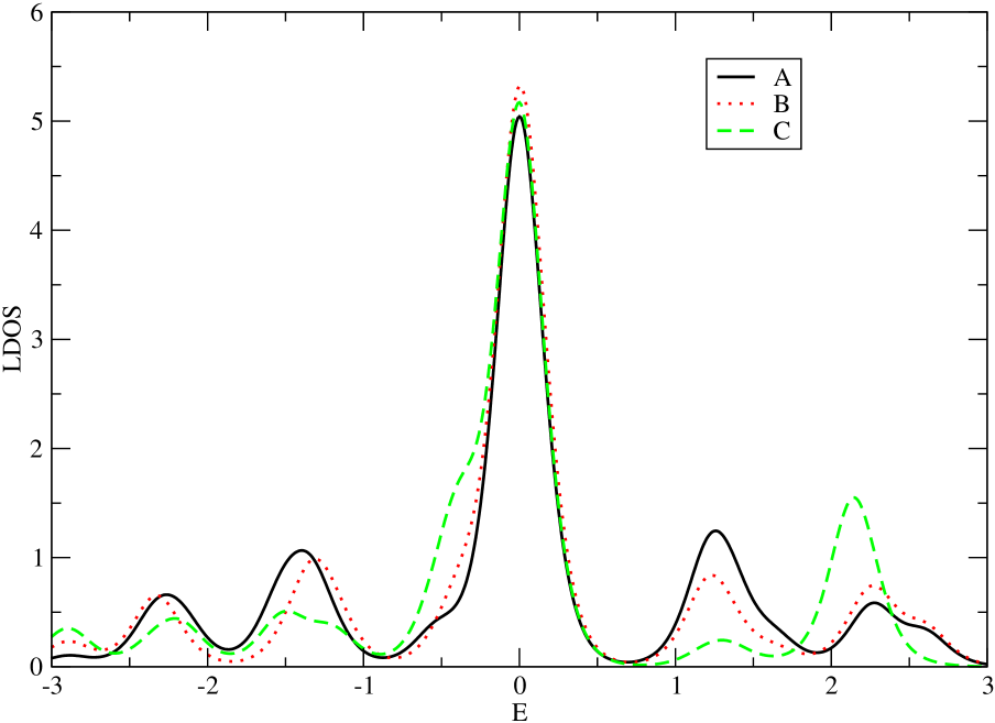
Figure 17: The LDOS for the points A,B,C that are seen in the figure 16 at the $(5,0)$ nanocone.

References

- (1) S. Iijima, Nature 354, 56 (1991).
- (2) J.W.G. Wildoer, L.C. Venema, A.G. Rinzler, R.E. Smalley, and C. Dekker, Nature 391, 59 (1998).
- (3) N. Stefanakis, Phys. Rev. B 70, 12502 (2004).
- (4) R.Saito, M. Fujita, G. Dresselhaus, M.S. Dresselhaus, Phys. Rev. B 391, 59 (1992).
- (5) E.N. Economou, Green’s functions in Quantum Physics Springer Verlag Series in Solid-State Sciences Vol. 7 (Springer Verlag, Berlin, 1979).
- (6) N. Stefanakis, Phys. Rev. B 66, 024514 (2002).
- (7) H. Jirari, R. Mélin, and N. Stefanakis, Eur. Phys. J. B 31, 125 (2003).
- (8) N. Stefanakis and R. Mélin J. Phys.: Condens. Matter 15, 3401 (2003).