Dynamical Alignment in Three Species Tokamak Edge Turbulence

Abstract

Three dimensional computations of self consistent three species gyrofluid turbulence are carried out for tokamak edge conditions. Profiles as well as disturbances in dependent variables are followed, running the dynamical system to transport equilibrium. The third species density shows a significant correlation with that of the electrons, regardless of initial conditions and drive mechanisms. For decaying systems the densities evolve toward each other. Companion tests with a simple two dimensional drift wave model show this persists even if the third species is a passively advected test field. Similarity in the transport character of electrons and the trace species does not imply that the electrons themselves have a test particle transport character.

I Introduction — Trace Species Transport

It is an interesting question whether the electrons and ions in a magnetically confined plasma are transported in the same way test particles in a randomly turbulent velocity field would be Horton (1985); Manfredi and Dendy (1997); Beyer et al. (1999); Basu et al. (2003). One might consider to investigate this by placing test particles or a trace species into an otherwise self consistent turbulence computation or experimentally by measuring trace species transport and comparing to the transport of the electrons Zastrow et al. (2004). Not only the transport coefficients are interesting, but also the basic character, namely, whether or not the transport is a random walk process Spineanu and Vlad (1997); Naulin et al. (1999); Annibaldi et al. (2000, 2002). It might be tempting to conclude that if the transport of the trace species were the same as that of the electrons, then the electrons themselves should be transported essentially randomly.

It is useful to provide a falsification constraint on this logic. Gradient driven transport in a magnetised plasma is usually very different from test particle transport in a fluid, due to the strong coupling between the electrostatic potential, which serves as the stream function for the ExB fluid velocity, and the electron density Hasegawa and Mima (1978); Wakatani and Hasegawa (1984); Scott (1990). The coupling is effected by the action of parallel currents and produces a strong correlation between the potential and density. Ultimately, if the electrons are adiabatic (Boltzmann relation vis-a-vis the potential) then there is no net transport of electrons even though there is turbulence, which could also be driven by the ion temperature Horton et al. (1980); Hamaguchi and Horton (1990); Dimits et al. (2000). Since ExB transport is ambipolar, it follows that there is also no net transport of ions (neglecting the small charge density implied by a finite ExB vorticity). Even in robustly electromagnetic tokamak edge turbulence, where the free energy comes from the extent to which the electrons are nonadiabatic, the adiabatic response is always of qualitative importance, and there is a strong correlation between the potential and the electron density Scott (1997, 2002).

What we will show herein is that in most reasonable circumstances the test particle species, even when it is a tracer field with vanishing influence upon the electrostatic potential, follows the same dynamics as the electron density. The process has a very similar appearance and results ultimately from the same mechanism as “dynamical alignment” between a passively advected density and the vorticity in neutral fluid turbulence Gang et al. (1991). It is a manifestation of (1) the advective nonlinearity being the most effective process in the equation for each quantity, and (2) each of these quantities having a strong direct cascade in its squared amplitude (playing the role of an entropy contribution) despite the fact that the flow energy has an inverse cascade Scott (1991). The basic nonlinear dynamics is sufficiently general that these cascade tendencies persist in the presence of strong, dissipative forcing Camargo et al. (1995). The result is that any initialised imprint on the spatial morphology of either variable is quickly transferred to small, dissipative scales, and the subsequent evolution, being the same for both quantities, produces similar morphology especially at scales within the inertial range of the turbulence.

The computations are done in three dimensional flux tube geometry, with a fully self consistent three species gyrofluid model Beer and Hammett (1996) with two ion species plus electrons, generalised to allow nonadiabatic, electromagnetic electron dynamics Scott (2000), but restricted to two moments per species in the “GEM3” model with clean energetics and clear correspondence to fluid edge turbulence models Scott (2003a). Not only the evolution of the small scale eddies are followed, but also that of the zonal profiles (flux surface averages, cf. Ref. Beyer et al. (1999)). This dynamics is followed to transport equilibrium for cases driven by a source, and for at least one transport decay time for cases with no sources. The trace ion species is initialised either the same as for the electrons (random bath disturbances plus a profile), or simply with a narrowly localised profile. In some cases both ion species are given equal background densities. In each case, the initial differences are eliminated by the evolution of the turbulence, and at late times the morphology of all species densities are closely similar, with a high degree of cross correlation between any two of them.

The main result is that even though the electrons are not transported passively, the density of a trace species is transported the same way as the electrons are. A companion test is given by a simple two dimensional drift wave model, following only the potential and electron density and their dissipative coupling Wakatani and Hasegawa (1984), plus an additional equation for a third field which is the density of a strict test particle species. Here, the regime of the electrons response is varied from deeply hydrodynamic to adiabatic Gang et al. (1991); Scott (1991). In either case, the test particle density closely follows the electron density, in all regimes, regardless of whether the electron and test particle densities are similarly or differently driven. This should serve as a caution against prematurely concluding that the density in a magnetised plasma are passively advected in the case the electrons and a trace impurity species should be observed to display the same transport properties.

Following sections document the GEM3 model as used, the results in decaying and driven cases, respectively, and the results from the dissipatively coupled, two dimensional model. A discussion and summary is given at the end.

II The Three Species GEM3 Model

For this study we use the GEM3 model, which allows a finite background temperature for all species but does not follow the dynamics of the temperatures or parallel heat fluxes Scott (2003a). It allows drift wave and ideal and resistive ballooning dynamics according to the parameters

$$\hat{\beta}={4\pi p_{e}\over B^{2}}\left(qR\over L_{\perp}\right)^{2}\qquad\qquad C=0.51{\nu_{e}\over c_{s}/L_{\perp}}{m_{e}\over M_{i}}\left(qR\over L_{\perp}\right)^{2}$$ (1)

controlling the parallel electron response and

$$\delta={\rho_{s}\over L_{\perp}}\qquad\qquad{\omega_{B}}=2{L_{\perp}\over R}$$ (2)

controlling the perpendicular drift dynamics and the magnetic curvature effects. Both interchange and geodesic curvature are retained Scott (2003b). Normalisation is in terms of a profile scale $L_{\perp}$ and the sound speed $c_{s}$, giving a natural drift frequency of $c_{s}/L_{\perp}$. The parallel dynamics is normalised in terms of $qR$, where the parallel connection length is $2\pi qR$, giving the $qR/L_{\perp}$ scale ratios in the parameters. The range of scales under consideration is everything between the drift scale $\rho_{s}$ and the profile scale $L_{\perp}$. The collisional drift wave regime is roughly $C>1$, becoming electromagnetic if $\hat{\beta}>1$. Ideal and resistive ballooning enter if $\hat{\beta}{\omega_{B}}>1$ or $C{\omega_{B}}>1$, respectively. The first two conditions are usually satisfied but the latter two are not. Hence, the principal physical process is drift Alfvén turbulence Scott (1997, 2002). Geodesic curvature is always important as its role is to regulate the attendant zonal ExB flows Scott (2003b).

The profiles as well as the fluctuations in the dependent variables are followed, so that transport as well as turbulence can be computed, even though the equations are still homogeneous in the normalised parameters. Each species is characterised by a background charge density, temperature/charge ratio, and mass/charge ratio, given by the normalised parameters

$$a_{z}={n_{z}Z/n_{e}}\qquad\qquad\tau_{z}={T_{z}/ZT_{e}}\qquad\qquad\mu_{z}={M_{z}/ZM_{D}}$$ (3)

in terms of a reference electron temperature $T_{e}$ and deuterium mass $M_{D}$. The scale ratio for the parallel dynamics comes in as $\epsilon_{z}=\mu_{z}(qR/L_{\perp})^{2}$. For electrons, $a_{e}=\tau_{e}=-1$ and $\mu_{e}=-(m_{e}/M_{D})$. For a single component deuterium plasma we would have $a_{i}=\mu_{i}=1$ and $\tau_{i}$ the nominal ion/electron temperature ratio $T_{i}/T_{e}$. With two ion species (the second labelled ’t’) we specify the three parameters independently for each species but then restrict to a neutral plasma by taking $a_{i}=1-a_{t}$. For simplicity we will assume a deuterium/tritium plasma with equal temperatures for all species.

The GEM3 model is given by moment equations for the density and parallel velocity of each species,

$${d_{z}\widetilde{n}_{z}\over dt}=-B\nabla_{\parallel}{\widetilde{u}_{z}{}_{\parallel}\over B}+{\cal K}\left(\widetilde{\phi}_{G}+\tau_{z}\widetilde{n}_{z}\right)$$ (4)

$$\hat{\beta}{\partial\widetilde{A}_{\parallel}\over\partial t}+\epsilon_{z}{d_{z}\widetilde{u}_{z}{}_{\parallel}\over dt}+C\widetilde{J}_{\parallel}=-\nabla_{\parallel}\left(\widetilde{\phi}_{G}+\tau_{z}\widetilde{n}_{z}\right)+{\cal K}\left(\epsilon_{z}\tau_{z}\widetilde{u}_{z}{}_{\parallel}\right)$$ (5)

including the effects of the toroidal magnetic drifts also in the parallel velocity moment equation Beer and Hammett (1996); Scott (2004). The ExB advective and parallel derivatives are given by

$${d_{z}\over dt}={\partial\over\partial t}+[\widetilde{\phi}_{G},]\qquad\qquad\nabla_{\parallel}={1\over B}{\partial\over\partial s}-[\hat{\beta}\widetilde{A}_{\parallel},]$$ (6)

in terms of a Poisson bracket defined by

$$[f,g]=\delta\left({\partial f\over\partial x}{\partial g\over\partial y}-{\partial f\over\partial y}{\partial g\over\partial x}\right)$$ (7)

noting the species-dependent nature of $\widetilde{\phi}_{G}$. The curvature operator and perpendicular Laplacian are given by

$${\cal K}=\delta{\omega_{B}}\left[\left(\cos s+g^{xy}_{k}\sin s\right){\partial\over\partial y_{k}}+\sin s{\partial\over\partial x}\right]\qquad\nabla_{\perp}^{2}=\delta^{2}\left[\left({\partial\over\partial x}+g^{xy}_{k}{\partial\over\partial y_{k}}\right)^{2}+{\partial^{2}\over\partial y_{k}^{2}}\right]$$ (8)

where $g^{xy}_{k}=\hat{s}[s-s_{k}]$ is the off diagonal metric element and $\hat{s}$ is the shear, and $y_{k}$ denotes the member of the family of field aligned coordinate systems which is orthogonal at $s=s_{k}$. The gyroaverage operator is defined by

$$\widetilde{\phi}_{G}=\Gamma_{0}^{1/2}(k_{\perp}^{2}\rho_{z}^{2})\widetilde{\phi}\qquad\qquad\rho_{z}^{2}={\mu_{z}\tau_{z}\over B^{2}}$$ (9)

with $\rho_{z}$ the species gyroradius in terms of the nominal $\rho_{s}$ and with $k_{\perp}^{2}$ the Fourier transform of $-\nabla_{\perp}^{2}$ (note $k_{\perp}^{2}$ contains the factor $\delta^{2}$). The electrostatic potential is determined by the gyrofluid analog Dorland and Hammett (1993) of the gyrokinetic Poisson equation Lee (1983),

$$\sum_{z}a_{z}\left[\Gamma_{0}^{1/2}\widetilde{n}_{z}+{\Gamma_{0}-1\over\tau_{z}}\widetilde{\phi}\right]=0$$ (10)

with $\Gamma_{0}$ always taking the argument $(k_{\perp}^{2}\rho_{z}^{2})$. The magnetic potential is determined by the gyrofluid Ampere’s law,

$$-\nabla_{\perp}^{2}\widetilde{A}_{\parallel}=\widetilde{J}_{\parallel}\qquad\qquad\widetilde{J}_{\parallel}=\sum_{z}a_{z}\widetilde{u}_{z}{}_{\parallel}$$ (11)

hence by the various velocity moments making up the parallel current.

All of this is in local flux tube geometry defined separately with respect to each drift plane ($xy_{k}$, defined globally, orthogonal at $s=s_{k}$), each on its own globally field aligned coordinate system, so that the linear parallel derivative ($\partial/\partial s$) incurs shifts in the $y$-direction to reflect the magnetic shear. The simplest version of the geometry is used, in which the metric of the coordinate system referenced to each drift plane is unit diagonal on that plane, and the magnetic field strength is $B=1$, giving the above Laplacian and curvature operators. This is the “shifted metric” treatment; for further detail see Ref. Scott (2001). Elsewhere, the subscript on $y_{k}$ is omitted (the form of the Poisson bracket is unaffected).

The equations are solved on a domain $L_{x}\times L_{y}\times L_{s}$, with $L_{s}=2\pi$ due to the global consistency constraint. The boundary conditions on the dependent variables in the drift plane are Dirichlet (vanishing value) at $x=L_{x}/2$ and Neumann (vanishing derivative) at $x=-L_{x}/2$, and periodic on $-L_{y}/2<y<L_{y}/2$, with the $x$-direction implemented in terms of the quarter-wave FFT so that the correct value of $\Gamma_{0}$ is obtained for each wavenumber. The boundary conditions on $s$ are defined by global consistency Scott (1998), on the interval $-\pi<s<\pi$, implemented using the shifted metric treatment Scott (2001).

The numerical scheme is one which has been used previously in three dimensional drift wave computation Naulin (2002). Poisson bracket structures in $xy$ are evaluated with a discretisation which preserves their properties Arakawa (1966). The linear $\partial/\partial s$ and ${\cal K}$ terms are evaluated using centred differences. The timestep is a third order scheme using both the dependent variables and their time derivatives to build the new dependent variables at the next time step Karniadakis et al. (1991). In contrast to most other methods, this scheme is stable to waves. Nevertheless, the direct thermal free energy cascade Gang et al. (1991); Scott (1991) creates the need for numerical dissipation at small scale Scott (2002). This is effected by a diffusion $-\nu_{\parallel}\partial^{2}/\partial s^{2}$ and a hyperdiffusion $\nu_{\perp}\nabla_{\perp}^{4}$ added to each ExB derivative (applying the dissipation to the moment variables but not directly to the fields). The spatial grid node count is $64\times 256\times 16$ in $xys$, on a domain given by $L_{y}=4L_{x}=80\pi\rho_{s}=4L_{\perp}$, or simply $4$ in normalised units, and $L_{s}=2\pi$. The minimum value of $k_{y}\rho_{s}$ is therefore $0.025$. The timestep is $\tau=0.05$, and runs are taken to approximately $t=2000$. The artificial dissipation coefficients are $\nu_{\parallel}=0.003$ and $\nu_{\perp}=0.002$.

III GEM3 Results for Decaying Cases

The first set of results under consideration is the decaying scenario: the domain is loaded with a density profile and density fluctuations, and the system is allowed to relax. Profile maintenance is restricted to a sink term on the right hand side of each density equation,

$${\partial\widetilde{n}_{z}\over\partial t}=\cdots-\oint{dy\over L_{y}}\,\widetilde{n}_{z}\,p(x)\qquad\qquad p(x)=0.3\exp\left[-{(x-L_{x}/2)^{2}\over(0.1\,L_{x})^{2}}\right]$$ (12)

where the integration denotes an average over $y$. Net transport in the direction $\nabla x$ into this sink then causes slow decay of the overall density profile (zonal average of $\widetilde{n}_{e}$).

The initial profiles are given by

$$n_{i0}={1\over 2}\left[1-\sin{\pi x\over L_{x}}\right]\qquad\qquad n_{t0}=\exp\left[-{x^{2}\over(0.1\,L_{x})^{2}}\right]$$ (13)

with

$$n_{e0}=(1-a_{t})n_{i0}+a_{t}n_{t0}$$ (14)

with subscripts $\{e,i,t\}$ referring to electrons, main ions, and trace ions, respectively, with $a_{t}$ the background charge density parameter of the trace ions. The electrons and main ions start with a random bath of fluctuations at nonlinear amplitude, $\widetilde{n}$, normalised such that the RMS level is $3.0\times\delta$, described elsewhere Scott (1990, 2001), with

$$\widetilde{n}_{e}=(1-a_{t})\widetilde{n}\qquad\qquad\widetilde{n}_{i}=\widetilde{n}\qquad\qquad\widetilde{n}_{t}=0$$ (15)

The trace ions start solely with their profile. The initial electrostatic potential is then given by Eq. (10).

The initial evolution is the excitation of “Pfirsch-Schlüter” profile modes, especially the global Alfvén oscillation. This is caused by the fact that the initial equilibrium is only one-dimensional while the actual one is two-dimensional, including Pfirsch-Schlüter currents and flows. It involves the “sideband modes” given by $\left\langle\widetilde{J}_{\parallel}\cos s\right\rangle$ and $\left\langle\widetilde{\phi}\sin s\right\rangle$, where the angle brackets denote the zonal average (over $y$ and $s$). These are excited by the action of the magnetic compression ${\cal K}$ upon the pressure profile $\left\langle p\right\rangle$, where $p=\sum_{z}a_{z}\tau_{z}\widetilde{n}_{z}$, due to the $\sin s$ term in ${\cal K}$ acting upon the $k_{y}=0$ component; in other words, the geodesic curvature. The decay of the global Alfvén oscillation proceeds through resistive dissipation, $C\left\langle\widetilde{J}_{\parallel}\cos s\right\rangle$. When these sideband modes reach dissipative equilibrium, the Pfirsch-Schlüter current is established. Over about the same time interval, $0<t<200$, the basic nonlinear drift wave mode structure is set up Scott (1997, 2002, 2003a). Parallel sound wave dynamics, the geodesic acoustic sideband dynamics, and the zonal flows all reach statistical equilibrium by about $t=1500$ Scott (2003b). For typical edge parameters the profile decay (i.e., transport) time scale is comparable to this, so we are dealing with a slowly transient case. However, it does provide a useful control against the effects of profile maintenance (driving of the densities using a source) upon the turbulence.

The standard case, reflecting typical tokamak edge conditions, is given by the parameters $\delta=0.0159$, $\hat{\beta}=1$, $C=2.5$, $\tau_{i}=1$, ${\omega_{B}}=0.05$, and $(qR/L_{\perp})^{2}=18350$. This very roughly corresponds to a physical parameter set of $n_{e}=3\times 10^{13}\,{\rm cm}^{-3}$, $T_{e}=100\,{\rm eV}$, $B=2.5\,{\rm T}$, $q=3.3$, $R=160\,{\rm cm}$, and $L_{\perp}=4\,{\rm cm}$. As noted above, we also use deuterium as the main ion species and tritium as the trace species, with $\tau_{t}=1$ and $\mu_{t}=1.5$ and $M_{D}/m_{e}=3670$, and either $a_{t}=0$ (strict test particles) or $a_{t}=0.1$ (minority species).

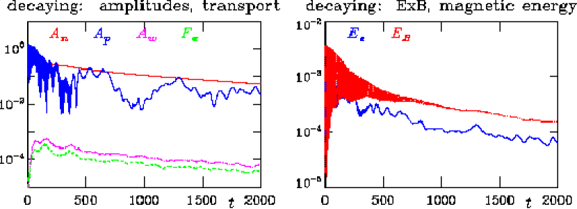
Figure 1: Time traces of free energy amplitudes and transport, showing initial saturation of the turbulence after $t=500$ and overall decay on a scale of about $1500$, all in units of $L_{\perp}/c_{s}$.

Selected time traces of the case with $a_{t}=0$ are shown in Fig. 1. In the left hand frame, the signal $A_{n}$ is the grid node average of $\sum_{z}a_{z}\tau_{z}\widetilde{n}_{z}^{2}/2$, giving the total thermal free energy, and $A_{p}$ is $\widetilde{\phi}^{2}/2$, tracking mostly the zonal flows, and $A_{w}$ is $\widetilde{\Omega}^{2}/2$, tracking mostly the activity of the turbulence, and $F_{e}$ is $\widetilde{n}_{e}\widetilde{v}_{E}^{x}$, the transport, with $\widetilde{v}_{E}^{x}=-\delta(\partial\widetilde{\phi}/\partial y)$. In the right hand frame, the signal $E_{e}$ is $\sum_{z}a_{z}\widetilde{\phi}_{G}\widetilde{n}_{z}/2$, the ExB energy, and $E_{B}$ is $\sum_{z}a_{z}\widetilde{A}_{\parallel}\widetilde{u}_{z}{}_{\parallel}/2$, the magnetic energy. Here, $\widetilde{\Omega}=-\sum_{z}a_{z}\widetilde{n}_{z}$ defines the generalised vorticity (at zero FLR it is just the ExB vorticity). The signature of $E_{e}$ and $E_{B}$ is that of the global Alfvén oscillation. The equilibrium is well established after about $t=250$. The other traces show that the overall statistical equilibration time of the turbulence and zonal flows is comparable to the transport decay time, and that the vorticity and transport track each other closely. By $t=1500$ the total amount of electrons, $\widetilde{n}_{e}$ integrated over the volume, has decayed by about half.

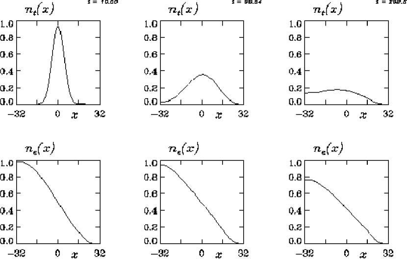
Figure 2: Profiles of the electron ($\widetilde{n}_{e}$) and trace ion ($\widetilde{n}_{t}$) densities at early times $t=10$ and $100$ and $300$ in the evolution. The initial value is unity in these units, and $x$ is in units of $\rho_{s}$. The trace ion profile is deconstructed by the turbulence and fills in.

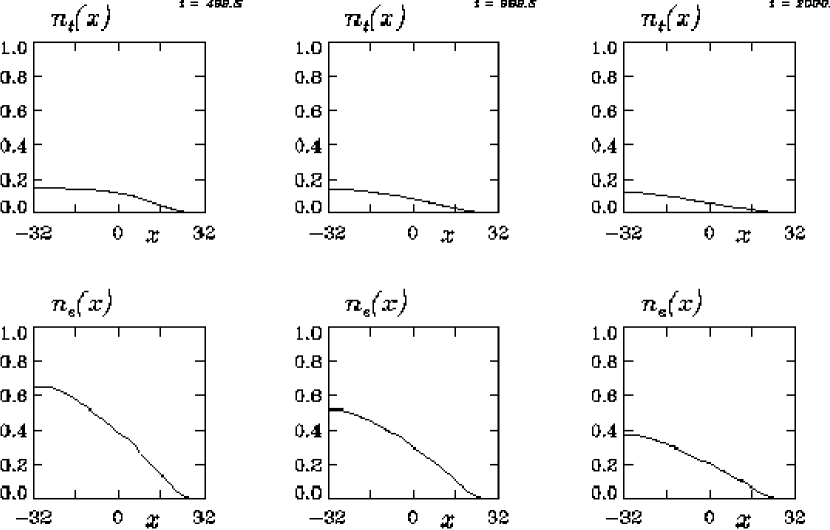
Figure 3: Profiles of the electron ($\widetilde{n}_{e}$) and trace ion ($\widetilde{n}_{t}$) densities at medium to late times $t=500$ and $1000$ and $2000$ in the evolution. The initial value is unity in these units, and $x$ is in units of $\rho_{s}$. When the value of the trace ion profile at the left boundary becomes the maximum, both profiles decay together.

The evolution of the decaying profiles (zonal averages, over all $y$ and $s$ for particular $x$) of the electron and trace densities is shown in Figs. 2 and 3. In these units, the maximal initial value is unity, and the first frame at $t=10$ shows that the turbulence is already deconstructing the initial profile of $\widetilde{n}_{t}$. The trace species distribution spreads until the value at $x=-L_{x}/2$ ($-32$ in units of $\rho_{s}$) rises from zero at $t=100$. Thereafter the trace profile fills in as the electron profile decays. When the value at $x=0$ reaches that at $x=-L_{x}/2$, the $\widetilde{n}_{t}$ profile itself begins to decay. At late times, the profiles of $\widetilde{n}_{e}$ and $\widetilde{n}_{t}$ are similar. As the driven cases discussed in the next Section will show, this behaviour is not indicative of a particle pinch in either species.

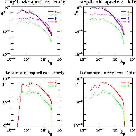
Figure 4: Spectra of selected quantities at early ($t=500$) and late ($t=1500$) stages of the turbulence, with $k_{y}$ in units of $\rho_{s}^{-1}$. Squared amplitudes of $\widetilde{\phi}$ and $\widetilde{n}_{e}$ and $\widetilde{n}_{t}$ and the vorticity $\widetilde{\Omega}$ are labelled by ‘p’ and ‘n’ and ‘z’ and ‘w’ respectively. The tendency of $\widetilde{\phi}$ and $\widetilde{n}_{e}$ to follow each other with $\widetilde{\Omega}$ much flatter is a basic signature of drift wave turbulence. The electron (‘n’) and trace ion (‘z’) transport fluxes also follow each other.

The most prominent amplitude/energy spectra (squared amplitudes, Fourier decomposed $y\rightarrow k_{y}$, averaged over $0<x<L_{x}/2$ and all $s$) are shown in Fig. 4, averaged over the intervals $500<t<600$ and $1500<t<1600$, respectively representing the early and late stages of the turbulence. These are reflective of typical drift wave mode structure as we expect in this regime; note especially that $\widetilde{n}_{e}^{2}$ as a function of $k_{y}$ (labelled $n$) follows $\widetilde{\phi}^{2}$ (labelled $p$) throughout the spectrum, as the average value of the parallel wavenumber $k_{\parallel}$ self adjusts to whatever is necessary for the parallel currents to balance the nonlinear excitation rates of the ExB vorticity. The vorticity spectrum itself, $\widetilde{\Omega}^{2}$ (labelled $w$), is much flatter, extending all the way to $k_{y}=1$ in units of $\rho_{s}^{-1}$. The transport spectrum, $\widetilde{n}_{e}\widetilde{v}_{E}^{x}$, also shown for both early and late stages, peaks at relatively low $k_{y}$ but is broadband. We find similarly standard drift wave mode structure results for the parallel envelopes and transport and energy transfer spectra, as presented in Refs. Scott (2002, 2003a), not shown here.

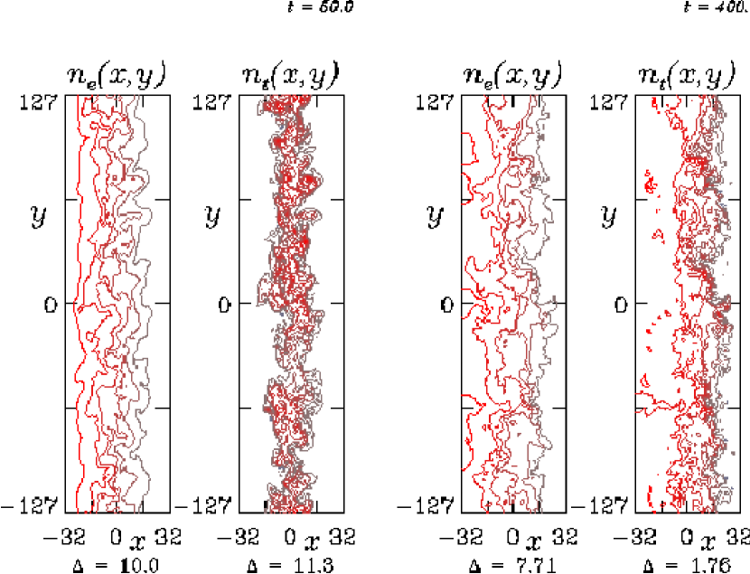
Figure 5: Spatial morphology of the electron ($\widetilde{n}_{e}$) and trace ion ($\widetilde{n}_{t}$) densities at $t=50$ and $400$, during saturation. The contour interval is shown in units of $\delta=0.0159$, and $x$ and $y$ are in units of $\rho_{s}$ in each case. Starting very different, their spatial forms evolve towards each other.

The spatial morphology at $t=50$ and $400$ is shown in Fig. 5, as contour patterns in the $xy$-plane at $s=0$. The form of $\widetilde{n}_{t}$ and $\widetilde{n}_{e}$ start out very differently owing to the initialisation. The spatial morphology however becomes quickly similar after the turbulence deconstructs the original profile of $\widetilde{n}_{t}$ (transfer free energy from $k_{y}=0$ to the entire $k_{y}$-spectrum). At $t=50$ the part of the contour distribution for $x>0$ is already very similar, even though the values at $x=-L_{x}/2$ are still close to zero. However, the spectra and even the spatial morphology evolve toward each other on all scales, including the profile scale. After $t=400$ they remain very close. The fact that the spectrum of $\widetilde{n}_{t}$ is slightly flatter on the smallest scales is reflected in the somewhat noisier form of the morphology of $\widetilde{n}_{t}$, seen most clearly in the outermost contour.

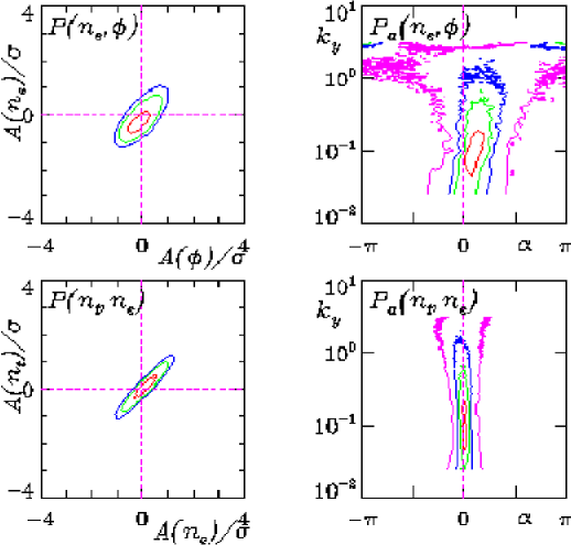
Figure 6: Cross correlation and phase shift distributions between the electron density ($\widetilde{n}_{e}$) and electrostatic potential ($\widetilde{\phi}$), and between the trace ion density ($\widetilde{n}_{t}$) and $\widetilde{n}_{e}$, averaged over the interval $500<t<1500$, with $k_{y}$ in units of $\rho_{s}^{-1}$, measured as described in Refs. Scott (1997, 2002). Note that $\widetilde{\phi}$ serves as the stream function for the turbulent ExB eddies. The first pair show the usual signature of drift wave mode structure (close correlation and small phase shifts at all wavelengths), while the second pair show the dynamical alignment between the trace ion and electron densities. This is the case with $a_{t}=0$; the one with $a_{t}=0.1$ was quantitatively very similar in all respects, as detailed in the text.

The closeness of $\widetilde{n}_{t}$ and $\widetilde{n}_{e}$ may be quantified by their cross correlation and phase shift distributions. These are more usually employed to evaluate the relation between $\widetilde{n}_{e}$ and $\widetilde{\phi}$, to distinguish between drift and MHD mode structure Scott (1997, 2002, 2003a)). An “adiabatic” relationship is characterised by a close cross correlation and a narrow phase shift distribution peaked near zero. A “hydrodynamic” relationship, the one expected of passive scalar advection in a neutral fluid, is characterised by a very weak or zero cross correlation and a wide phase shift distribution centred upon $\pi/2$, the value which gives energetically maximum gradient drive. The fields in question are sampled on the $xy$-plane at $s=0$, with the $k_{y}=0$ mode stripped out, over the interval $500<t<1500$ with the turbulence saturated and still well developed, and for $5<x<27$ to keep clear of the outer boundary sink region and remain in the gradient region for $\widetilde{n}_{t}$. These diagnostics are shown for both $\{\widetilde{n}_{e},\widetilde{\phi}\}$ and $\{\widetilde{n}_{t},\widetilde{n}_{e}\}$ in Fig. 6. The first pair show close correlation (overall: $0.721$) and low phase shifts (positive, narrowly distributed, below $\pi/4$) indicative of drift wave mode structure. The second pair shows extremely tight correlation (overall: $0.937$) and a narrow phase shift distribution centred upon zero.

The expected form for a passive scalar quantity completely uncoupled to the potential would be hydrodynamic, with random phase shifts in a case with no gradient. By contrast, although in the dynamical equations there is no direct coupling between $\widetilde{n}_{e}$ and $\widetilde{n}_{t}$, they are very closely correlated and their phase shift distribution is narrow and peaked at zero for every nonzero $k_{y}$ in the spectrum. Taking the two combinations from this figure together, we find that the electron and trace ion density fluctuations track each other very closely, despite the fact that the electrons themselves are not in a passive advection relationship to the ExB eddies. This is the phenomenon we refer to as “dynamical alignment” and the center of the phase shift distribution (essentially zero) and the value of the overall cross correlation (larger than $0.9$) give it a quantitative basis.

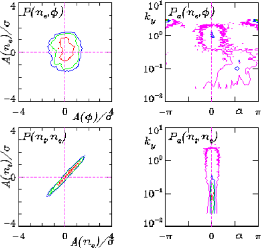
Figure 7: Cross correlation and phase shift distributions between the electron density ($\widetilde{n}_{e}$) and electrostatic potential ($\widetilde{\phi}$), and between the trace ion density ($\widetilde{n}_{t}$) and $\widetilde{n}_{e}$, for the case with $a_{t}=0.1$ and $\hat{\beta}=5$, averaged over the interval $500<t<800$, with $k_{y}$ in units of $\rho_{s}^{-1}$. The first pair now shows the high-beta ideal ballooning mode structure (very low correlation and phase shifts near $\pi/2$). The second pair shows the dynamical alignment between the trace ions and the electrons. Compare to Fig. 6. The dynamical alignment persists regardless of the actual character of the electron transport itself.

Testing against the presence and absence of a back reaction of $\widetilde{\phi}$ to $\widetilde{n}_{t}$, this basic case with $\hat{\beta}=1$ and $a_{t}=0$ was run again with $a_{t}=\{0.1,0.2,0.3,0.5\}$. The same results as presented above for $a_{t}=0$ were found, with the cross correlation values for $a_{t}=0.1$ given by $0.763$ for $\widetilde{n}_{e}$ and $\widetilde{\phi}$ and $0.947$ for $\widetilde{n}_{t}$ and $\widetilde{n}_{e}$, respectively. Cases with $\hat{\beta}=5$ with $a_{t}=0$ and $0.1$ were also run, looking for changes closer to the MHD regime in which the mode structure should be more hydrodynamic. The basic mode structure shows the changes resulting from the stronger role of the vortices at $k_{y}\rho_{s}=0.05$ to $0.1$ (convective cell modes on the scale of $L_{\perp}$), which in the $k_{y}$-spectra sit higher above the broadband drift wave turbulence and show much larger phase shifts. Nevertheless, the same closeness of $\widetilde{n}_{t}$ to $\widetilde{n}_{e}$ is found. The cross correlation and phase shift information as in the nominal case are shown in Fig. 7 for the case with $\hat{\beta}=5$ and $a_{t}=0.1$. The fact that this case is in the MHD regime is shown by the hydrodynamic relationship between $\widetilde{n}_{e}$ and $\widetilde{\phi}$; the overall cross correlation value is $-0.0259$. The persistence of the dynamical alignment is shown by the relationship between $\widetilde{n}_{t}$ and $\widetilde{n}_{e}$, which gives zero phase shifts and a overall cross correlation of $0.986$.

Regardless of the closeness of the relationship between $\widetilde{n}_{e}$ and $\widetilde{\phi}$, which varies with parameters (in this case $\hat{\beta}$ and $C$), the correlation between $\widetilde{n}_{e}$ and $\widetilde{n}_{t}$ is close to unity and the phase shifts are close to zero. Clearly, $\widetilde{n}_{t}$ is following $\widetilde{n}_{e}$ regardless of the latter’s relationship to $\widetilde{\phi}$.

What we now have to do is to determine the extent to which this result might be a fortuitous consequence of how the model is set up. To this end, we compare to driven cases run to transport equilibrium in the next Section, and then evaluate the phenomenon more fundamentally by studying the simplest dissipative drift wave model in the adiabatic and hydrodynamic limits, in the Section after that.

IV GEM3 Results for Driven Cases

We now turn to cases in which the profiles are maintained by sources so that the runs may be carried for arbitrary time. The setup is exactly as for the decaying cases, with the addition of the drive term

$${\partial\widetilde{n}_{z}\over\partial t}=\cdots+S_{z}(x)$$ (16)

for each density variable. Typically we use $S_{i}=S_{e}$ so as not to drive vorticity on the inner boundary. The basic profile source term has the shape of a Gaussian with $1/e$-width $0.3L_{x}$ centred upon $x=-L_{x}/2$ and a time constant chosen to anticipate the transport time scale. Narrower main source profiles (width $0.1L_{x}$) with correspondingly larger coefficients (i.e., at constant total source) were found to excessively excite artificial MHD modes. The trace ion source was centred upon $x=0$ to set up a gradient region for $x>0$ and to look for a pinch (finite gradient with no interior source) in the $x<0$ region, so $n_{t0}$ was used as a template. The source terms were chosen as

$$S_{e}=S_{i}=s_{e}\exp\left[-{(x+L_{x}/2)^{2}\over(0.3\,L_{x})^{2}}\right]\qquad\qquad S_{t}=s_{t}n_{t0}$$ (17)

for electrons, main ions, and trace ions, respectively. The parameters $s_{e}$ and $s_{t}$ are free; nominally they are both set to $10^{-3}$.

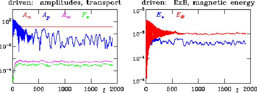
Figure 8: Time traces of free energy amplitudes and transport, showing initial saturation of the turbulence after $t=500$ and equilibration of the zonal flows and transport after about $t=1000$, all in units of $L_{\perp}/c_{s}$.

The standard case is the same as the one from the previous Section, with $a_{t}=0$, so that the trace ions are proper test particles. The same time traces are shown in Fig. 8, which can be compared to Fig. 1. The amplitudes and transport, in the left hand frame, show that the dynamics is well saturated after $t=1000$, so that late time averaged diagnostics are taken over the interval $1000<t<2000$. The time traces of the ExB and magnetic energies, labelled $E_{e}$ and $E_{B}$, respectively, are shown in the right hand frame, indicating that the global Alfvén oscillation damps away well before the saturated stage. The short time scale visible in the $A_{p}$ signal is indicative of the geodesic acoustic oscillation. The long time scale oscillation from the decaying case is absent in this figure, showing that it is a response to the overall profile decay in the other case.

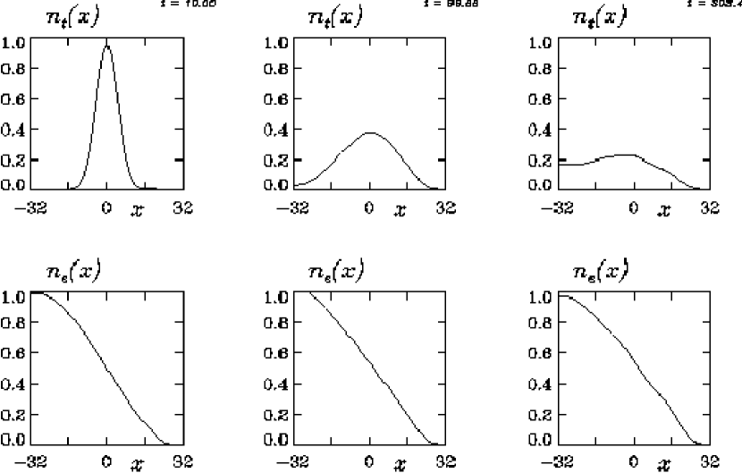
Figure 9: Profiles of the electron ($\widetilde{n}_{e}$) and trace ion ($\widetilde{n}_{t}$) densities at early times $t=10$ and $100$ and $300$ in the evolution. The initial value is unity in these units, and $x$ is in units of $\rho_{s}$. The trace ion profile is deconstructed by the turbulence and fills in.

The evolution of the profiles of the electron and trace densities in this driven case is shown in Figs. 9 and 10, measured the same way as in Figs. 2 and 3, for the decaying case. In these units, the maximal initial value is unity, and the first frame at $t=10$ shows that the turbulence is already deconstructing the initial profile of $\widetilde{n}_{t}$. Up until $t=100$ the evolution is the same as in the decaying case. The trace species distribution spreads until the value at the left boundary ($x=-32$ in units of $\rho_{s}$) is as large as that at the source ($x=0$). Transport equilibration, the temporal convergence of these profiles, sets in after $t=1000$. At late times, the profiles of $\widetilde{n}_{e}$ and $\widetilde{n}_{t}$ are similar outside the source regions. The flatness of $\widetilde{n}_{t}$ for $x<0$ is indicative of the absence of an impurity pinch. For this we note however that temperature disturbance and gradient dynamics is not followed, so there remains the possibility of an impurity pinch driven by the ion temperature gradient. Nevertheless, the background temperatures of the three species are equal, so this does show that the existence of warm ions does not by itself lead to an impurity pinch nor does the trace and main ion temperature lead to a “neoclassical” pinch, the underlying dynamics of which would indeed be contained in this model (geodesic curvature acting on the gradients through diamagnetic fluxes, and the interaction of this with parallel flows in the axisymmetric part of the dynamics).

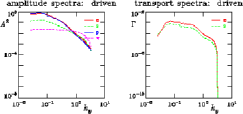
Figure 11: Spectra of amplitudes and transport in the saturated stage $1000<t<2000$, with $k_{y}$ in units of $\rho_{s}^{-1}$. Squared amplitudes of $\widetilde{\phi}$ and $\widetilde{n}_{e}$ and $\widetilde{n}_{t}$ and the vorticity $\widetilde{\Omega}$ are labelled by ‘p’ and ‘n’ and ‘z’ and ‘w’ respectively. The tendency of $\widetilde{\phi}$ and $\widetilde{n}_{e}$ to follow each other with $\widetilde{\Omega}$ much flatter is a basic signature of drift wave turbulence. The electron (‘n’) and trace ion (‘z’) transport fluxes also follow each other.

The spectra of the amplitudes and transport are shown in Fig. 11, averaged over the saturated stage, given by the interval $1000<t<2000$. These show the amplitudes of $\widetilde{n}_{e}$ and $\widetilde{\phi}$ peaking at large scales ($k_{y}<0.1$ in units of $\rho_{s}^{-1}$), while the transport is broadband almost all the way to $k_{y}=1$. The vorticity is flat to $k_{y}=1$. All of these are indicative of drift wave mode structure. The spectrum of $\widetilde{n}_{t}$ follows $\widetilde{n}_{e}$.

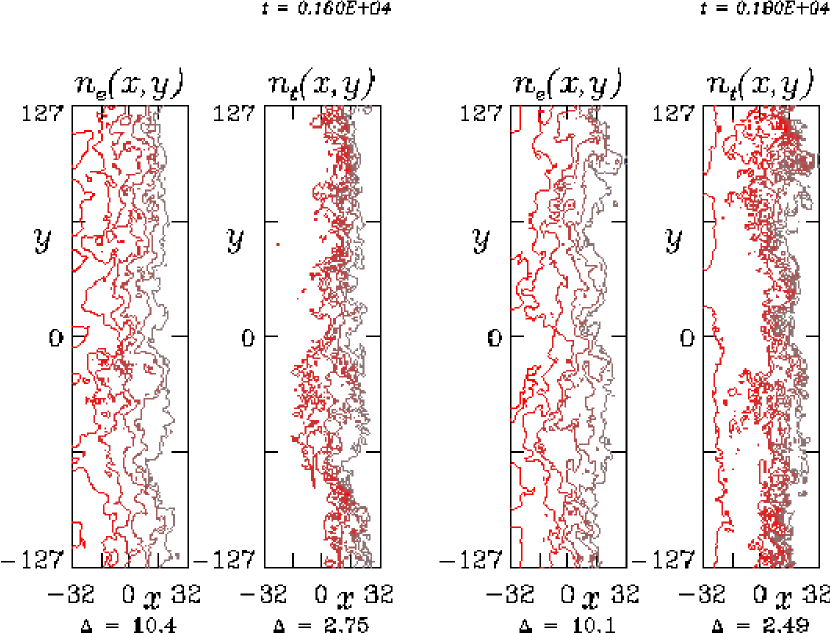
Figure 12: Spatial morphology of the electron ($\widetilde{n}_{e}$) and trace ion ($\widetilde{n}_{t}$) densities at two different times near the end of the run. The contour interval is shown in units of $\delta=0.0159$, and $x$ and $y$ are in units of $\rho_{s}$ in each case. Starting very different, their spatial forms track each other closely in saturation.

The spatial morphology at $t=2000$ is shown in Fig. 12, as contour patterns in the $xy$-plane at $s=0$. The form of $\widetilde{n}_{e}$ and $\widetilde{n}_{t}$ are closely similar. The fact that the spectrum of $\widetilde{n}_{t}$ is slightly flatter on the smallest scales is reflected in the somewhat noisier form of the morphology of $\widetilde{n}_{t}$, seen most clearly in the outermost contour. From time to time a small scale structure appears in $\widetilde{n}_{t}$ which is not reflected in $\widetilde{n}_{e}$, but the occurrences are rare enough not to affect the statistical result.

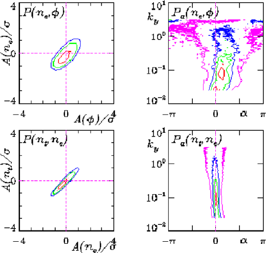
Figure 13: Cross correlation and phase shift distributions between the electron density ($\widetilde{n}_{e}$) and electrostatic potential ($\widetilde{\phi}$), and between the trace ion density ($\widetilde{n}_{t}$) and $\widetilde{n}_{e}$, for the driven case with $a_{z}=0.1$, averaged over the saturated stage $1000<t<2000$, with $k_{y}$ in units of $\rho_{s}^{-1}$, measured as described in Refs. Scott (1997, 2002). Compare with Fig. 6. Provided the sampling is done exterior to the source region, the results are the same. In particular, the drift wave mode structure signature remains whether or not the turbulence is “ambient” or “source driven”.

The cross coherence and phase shifts between $\widetilde{n}_{e}$ and $\widetilde{\phi}$ and between $\widetilde{n}_{t}$ and $\widetilde{n}_{e}$ are shown in Fig. 13, sampled over the saturated stage the same way as in the decaying case. The first pair show that the signature of drift wave mode structure (overall cross correlation: $0.674$) is not affected by the proximity of the source. For realistic drive levels there is therefore no qualitative difference between “ambient” and “source driven” turbulence, provided the physical separation of scales is well reproduced in the computations (note that a transport equilibration time of $1000$ with tokamak edge values of $L_{\perp}/c_{s}$ is already very short). The second pair show that the presence of the source just to the left of the measured region does not affect the dynamical alignment result (overall cross correlation: $0.920$), as can be judged by comparing with Fig. 6. But if this is measured over the whole radial domain, then the effect of not only the source but also the region interior to it is found to be large. So the conclusion of dynamical alignment between these two disturbance fields does depend on the relative strength of the nonlinear dynamics.

Having now determined that the three dimensional model recovers the same basic result in source free gradient regions, whether or not it is driven or allowed to decay, we now turn to the simplest two dimensional dissipative drift wave model for further comparison.

V Results in a Simple 2D Drift Wave Model

We distill the central physics behind the above results by comparing them to those from a simple two dimensional Hasegawa Wakatani drift wave model Wakatani and Hasegawa (1984), augmented by a continuity equation for a test species. The equations are

$${\partial\widetilde{\Omega}\over\partial t}+{\bf v}_{E}\cdot\nabla\widetilde{\Omega}=D\left(\widetilde{\phi}-\widetilde{n}_{e}\right)-{\cal K}\left(\widetilde{n}_{e}\right)+\nu_{d}\widetilde{\phi}$$ (18)

$${\partial\widetilde{n}_{e}\over\partial t}+{\bf v}_{E}\cdot\nabla\left(\widetilde{n}_{e}+n_{e}\right)=D\left(\widetilde{\phi}-\widetilde{n}_{e}\right)+{\cal K}\left(\widetilde{\phi}-\widetilde{n}_{e}\right)$$ (19)

$${\partial\widetilde{f}\over\partial t}+{\bf v}_{E}\cdot\nabla\left(\widetilde{f}+f\right)=0$$ (20)

for disturbances in the ExB vorticity, electron density, and test particle density, respectively. The domain is a single $xy$ drift plane, doubly periodic. Background gradient drive terms appear for both the electrons ($n_{e}$) and test particles ($f$); their $x$-derivatives yield the background gradients. The ExB advective derivative and vorticity are given by

$${\bf v}_{E}\cdot\nabla=\left({\partial\widetilde{\phi}\over\partial x}{\partial\over\partial y}-{\partial\widetilde{\phi}\over\partial y}{\partial\over\partial x}\right)\qquad\qquad\widetilde{\Omega}=\nabla_{\perp}^{2}\widetilde{\phi}$$ (21)

The dissipative coupling parameter $D$ serves as a model for the adiabatic response. The hydrodynamic and adiabatic limits are $D\rightarrow 0$ and $D\rightarrow\infty$, respectively. For $D=0$ the electrons and test particles have the same equation. For $D>1$ they are obviously very different. A simple interchange curvature model with ${\cal K}={\omega_{B}}\partial/\partial y$ and a long-wave damping coefficient $\nu_{d}$ are included to study saturated interchange turbulence. Note that this model uses the traditional “gyro-Bohm” local normalisation, with the factor of $\delta$ folded into the amplitudes.

For the purposes of this test series, the zonal flow question is avoided by setting temporal changes to the $k_{y}=0$ component of $\widetilde{\Omega}$ to zero. The Colella Colella (1990)/Van LeerLeer (1979) MUSCL scheme is applied to $d/dt$ as in previous versions of the 3D electromagnetic gyrofluid modelScott (2000) (the linear drive terms are combined into this, e.g., by defining $N=\widetilde{n}_{e}+n_{e}$). The terms involving $D$ are done via the implicit scheme of previous 2D drift wave models Scott (1988). In this, $D$ is applied only to the $k_{y}\neq 0$ components. The background profiles are chosen differently, with $\partial n_{e}/\partial x=-1$ and $\partial f/\partial x=-\omega_{z}\cos\pi x/L_{x}$ so that $\widetilde{n}_{e}$ and $\widetilde{f}$ are driven differently regardless of the value of the gradient parameter $\omega_{z}$. The domain size is given by $L_{x}=L_{y}=2\pi/K$, with $K$ nominally set to $0.1$ along with nominal values of $D=0.1$ and $\omega_{z}=1$. There are $64\times 64$ grid nodes for all cases. The timestep is set to $\tau=0.05$. All runs which reached saturation were taken to $t=1000$ with the interval $400<t<1000$ as the saturated stage.

The variations for the drift wave cases with ${\omega_{B}}=\nu_{d}=0$ were $D=\{0.001,0.003,0.01,0.03,0.1,0.3,1.,3.\}$ with nominal $K$ and $\omega_{z}$, $K=\{0.025,0.05,0.1\}$ at $D=0.01$ and nominal $\omega_{z}$, and $\omega_{z}=\{0.1,0.2,0.5,1.\}$ at nominal $D$ and $K$. The cases with $D=0.001$ and $0.003$ did not saturate, as thin radial flow jets formed and simply grew, so another scan with $D=\{0.001,0.003,0.01\}$ was done at $K=0.025$ and nominal $\omega_{z}$. In all cases in which saturation was found, the cross correlation between $\widetilde{\phi}$ and $\widetilde{n}_{e}$ was larger than $0.85$. This is due to the nature of the turbulence in this model: at low $D$ the spectrum migrates to large enough scale that $D$ can compete with $k_{\perp}^{2}\omega$, with $\omega$ close to the diamagnetic value of $k_{y}$, thereby guaranteeing strong adiabatic coupling for the long-wave side of the energy containing range. At high $D$, with all energetic transfer phenomena becoming weak at large scale, the turbulence again migrated there, and with the weak nonlinearities the cases for $D>1$ are strongly adiabatic with most of the energy again at long wavelength; the $D=3.0$ case was taken to $t=4000$ with the saturation stage taken as the $2000<t<4000$ interval. All of this has been the subject of previous study Wakatani and Hasegawa (1984); Camargo et al. (1995).

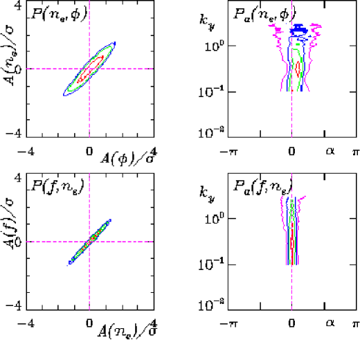
Figure 14: Control check using the nominal case from the 2D dissipative drift wave model with a test particle density field $\widetilde{f}$. Cross correlation and phase shift distributions, with $k_{y}$ in units of $\rho_{s}^{-1}$, between the electron density ($\widetilde{n}_{e}$) and the electrostatic potential ($\widetilde{\phi}$), and between $\widetilde{f}$ and $\widetilde{n}_{e}$. The first pair shows the drift wave mode structure and the second pair shows the dynamical test density alignment.

Regardless of any of this behaviour, the main point of this present study remained. The cross correlation between $\widetilde{n}_{e}$ and $\widetilde{f}$ was measured at $0.984$ or larger for all cases. For $D=0.01$ and larger at nominal $K$ and $\omega_{z}$ these correlation values were $\{0.999,0.998,0.992,0.985,0.984,0.987\}$ respectively. For $\omega_{z}=0.1$ and larger at nominal $D$ and $K$ all values were identical at $0.992$. For $K=0.025$ and larger at $D=0.01$ and nominal $\omega_{z}$ they were $\{0.998,0.9994,0.999\}$. For $D=0.001$ and larger at $K=0.025$ and nominal $\omega_{z}$ they were $\{0.99995,0.9998,0.998\}$. The cross correlation and phase shift distributions between $\widetilde{n}_{e}$ and $\widetilde{\phi}$ and between $\widetilde{f}$ and $\widetilde{n}_{e}$ are shown in Fig. 14 for the nominal case. The first pair show the expected near-adiabatic drift wave mode structure and the second pair show very close correlation between the densities.

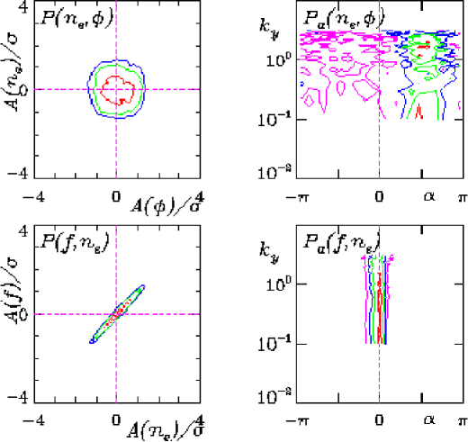
Figure 15: A further control check using the 2D interchange model with a test particle density field $\widetilde{f}$. Cross correlation and phase shift distributions, with $k_{y}$ in units of $\rho_{s}^{-1}$, between the electron density ($\widetilde{n}_{e}$) and the electrostatic potential ($\widetilde{\phi}$), and between $\widetilde{f}$ and $\widetilde{n}_{e}$. The first pair shows hydrodynamic mode structure and the second pair shows the dynamical test density alignment.

The purely hydrodynamic limit is found by setting $D=0$ and then ${\omega_{B}}=0.1$ to drive interchange turbulence and $\nu_{d}=0.01$ to allow it to saturate. The cross correlation and phase shift distributions for this case between $\widetilde{n}_{e}$ and $\widetilde{\phi}$ and between $\widetilde{f}$ and $\widetilde{n}_{e}$ are shown in Fig. 15. The first pair show the expected hydrodynamic mode structure and the second pair show very close correlation between the densities.

The phenomena of dynamical alignment therefore remained for all cases, surviving the control check represented by this simple 2D drift wave/interchange model.

VI Conclusions

A set of three dimensional computations of turbulence in an electromagnetic drift wave regime commensurate with tokamak edge turbulence of a fully self consistent, two-component plasma has been given. The principal focus has been on the second ion species as a proper test species, namely, with no back reaction on the polarisation, as controlled by a background charge density parameter nominally set to zero. Variation of this parameter was found to produce negligible changes. Both decaying and source driven cases were considered. This difference also produced no difference in turbulence regime, though with the sources present the turbulence and transport were able to fully saturate, leaving more activity at very small scale at late times. A set of two dimensional computations within a dissipative drift wave model with a test species continuity equation was also given as a control case. The numerical schemes and boundary conditions in the 2D and 3D models were different. Nevertheless, the same conclusion with regard to the correlation of the test ion species was always the same: the test ion and electron densities were found to be correlated to much better than 80 percent in all cases, and better than 90 percent in most, as measured outside the source region in the 3D driven cases.

It is important to note that the relationship between the electron density itself and the electrostatic potential (the stream function for the ExB eddies) was itself quite different among some of these cases. The adiabatic response of the potential back to the electrons is parameter dependent, with the electrons usually not in a test particle relationship vis-a-vis the eddies. Nevertheless, so long as there is a significant nonadiabatic electron density response, the test particle transport was found to conform to whatever the electron transport result was.

Indeed, these result suggest that the character of the adiabatic response is not the electrons following the potential, but the other way around: the potential pushes all species similarly through ExB advection, but the form of its disturbances and hence the ExB eddies follows that of the electron pressure disturbances due to the adiabatic response. The similarity of transport of all species regardless of fractional composition now becomes an expected result, since the ExB advection is the most robust effect in any of the continuity equations. The adiabatic response is therefore mostly a matter of the parallel current mediating the dynamics of polarisation.

There is an important experimental implication in this: Experiments are underway to measure the transport of trace tritium ions in tokamaks Zastrow et al. (2004). Transport of the trace ions is to be compared to that of the electrons. It is very important to note that if the two transports are found to have the same character, it does not follow that the electrons themselves transport like test particles, namely, that they should follow a random walk process. The existence of adiabatic coupling makes the electron transport different from this. The results in this work show that the potential finding that trace ion transport would be similar to the electron transport does not by itself give an indication of the character of the electron transport itself.

It remains to establish what these dynamical relationships become in a regime where the passing electrons are completely adiabatic, and particle transport is solely due to trapped electrons, and thermal transport is mostly due to the ions, through the standard ITG scenario which receives most current attention Dimits et al. (2000). Moreover, the question of an impurity driven particle pinch remains open, since the actual temperature fluctuation and gradient dynamics is not included in the GEM3 model. Future manifestations of this work will address these questions with a more detailed model Scott (2004) designed to treat them in either edge or core plasma regimes.

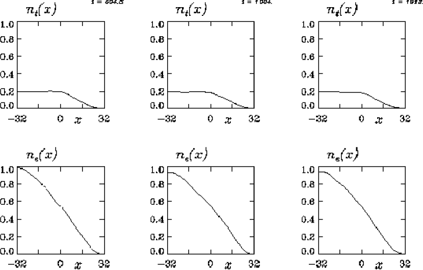
Figure 10: Profiles of the electron ($\widetilde{n}_{e}$) and trace ion ($\widetilde{n}_{t}$) densities at medium to late times $t=500$ and $1000$ and $2000$ in the evolution. The initial value is unity in these units, and $x$ is in units of $\rho_{s}$. Transport equilibration occurs after about $t=1000$.

References

- Horton (1985) W. Horton, Plasma Phys. Contr. Fusion 27, 937 (1985).
- Manfredi and Dendy (1997) G. Manfredi and R. O. Dendy, Phys. Plasmas 4, 628 (1997).
- Beyer et al. (1999) P. Beyer, Y. Sarazin, X. Garbet, P. Ghendrih, and S. Benkadda, Plasma Phys. Contr. Fusion 41, A757 (1999).
- Basu et al. (2003) R. Basu, T. Jessen, V. Naulin, and J. J. Rasmussen, Phys. Plasmas 10, 2696 (2003).
- Zastrow et al. (2004) K.-D. Zastrow, J. M. Adams, Y. Baranov, P. Belo, L. Bertalot, J. H. Brzozowski, C. D. Challis, S. Conroy, M. de Baar, P. de Vries, et al., Plasma Phys. Contr. Fusion 46, B255 (2004).
- Spineanu and Vlad (1997) F. Spineanu and M. Vlad, Phys. Plasmas 4, 2106 (1997).
- Naulin et al. (1999) V. Naulin, A. H. Nielsen, and J. J. Rasmussen, Phys. Plasmas 6, 4575 (1999).
- Annibaldi et al. (2000) S. V. Annibaldi, G. Manfredi, R. O. Dendy, and L. O. Drury, Plasma Phys. Contr. Fusion 42, L13 (2000).
- Annibaldi et al. (2002) S. V. Annibaldi, G. Manfredi, and R. O. Dendy, Phys. Plasmas 9, 791 (2002).
- Hasegawa and Mima (1978) A. Hasegawa and K. Mima, Phys. Fluids 21, 87 (1978).
- Wakatani and Hasegawa (1984) M. Wakatani and A. Hasegawa, Phys. Fluids 27, 611 (1984).
- Scott (1990) B. Scott, Phys. Rev. Lett. 65, 3289 (1990), expanded version in Phys. Fluids B 4 (1992) 2468.
- Horton et al. (1980) W. Horton, R. D. Estes, and D. Biskamp, Plasma Phys. 22, 663 (1980).
- Hamaguchi and Horton (1990) S. Hamaguchi and W. Horton, Phys. Fluids B 2, 1833 (1990).
- Dimits et al. (2000) A. M. Dimits, G. Bateman, M. A. Beer, B. I. Cohen, W. Dorland, G. W. Hammett, C. Kim, J. E. Kinsey, M. Kotschenreuther, A. H. Kritz, et al., Phys. Plasmas 7, 969 (2000).
- Scott (1997) B. Scott, Plasma Phys. Contr. Fusion 39, 1635 (1997).
- Scott (2002) B. Scott, New J. Phys. 4, 52 (2002).
- Gang et al. (1991) F. Y. Gang, P. H. Diamond, J. A. Crotinger, and A. E. Koniges, Phys. Fluids B 3, 955 (1991).
- Scott (1991) B. Scott, Phys. Fluids B 3, 51 (1991).
- Camargo et al. (1995) S. Camargo, D. Biskamp, and B. Scott, Phys. Plasmas 2, 48 (1995).
- Beer and Hammett (1996) M. A. Beer and G. Hammett, Phys. Plasmas 3, 4046 (1996).
- Scott (2000) B. Scott, Phys. Plasmas 7, 1845 (2000).
- Scott (2003a) B. Scott, Plasma Phys. Contr. Fusion 45, A385 (2003a).
- Scott (2003b) B. Scott, Phys. Lett. A 320, 53 (2003b), eprint arXiv:physics.plasm-ph/0208026.
- Scott (2004) B. Scott, Gem – an energy conserving electromagnetic gyrofluid model (2004), submitted to Phys. Plasmas, eprint arXiv:physics.plasm-ph/0501124.
- Dorland and Hammett (1993) W. Dorland and G. Hammett, Phys. Fluids B 5, 812 (1993).
- Lee (1983) W. W. Lee, Phys. Fluids 26, 556 (1983).
- Scott (2001) B. Scott, Phys. Plasmas 8, 447 (2001).
- Scott (1998) B. Scott, Phys. Plasmas 5, 2334 (1998).
- Naulin (2002) V. Naulin, New J. Phys. 4, 28 (2002).
- Arakawa (1966) A. Arakawa, J. Comp. Phys. 1, 119 (1966), repr. vol 135 (1997) 103.
- Karniadakis et al. (1991) G. E. Karniadakis, M. Israeli, and S. A. Orszag, J. Comp. Phys. 97, 414 (1991).
- Colella (1990) P. Colella, J. Comp. Phys. 87, 171 (1990).
- Leer (1979) B. V. Leer, J. Comp. Phys. 32, 101 (1979).
- Scott (1988) B. Scott, J. Comp. Phys. 78, 114 (1988).