Networks as Renormalized Models for Emergent Behavior in Physical Systems

Abstract

Networks are paradigms for describing complex biological, social and technological systems. Here I argue that networks provide a coherent framework to construct coarse-grained models for many different physical systems. To elucidate these ideas, I discuss two long-standing problems. The first concerns the structure and dynamics of magnetic fields in the solar corona, as exemplified by sunspots that startled Galileo almost 400 years ago. We discovered that the magnetic structure of the corona embodies a scale free network, with spots at all scales. A network model representing the three-dimensional geometry of magnetic fields, where links rewire and nodes merge when they collide in space, gives quantitative agreement with available data, and suggests new measurements. Seismicity is addressed in terms of relations between events without imposing space-time windows. A metric estimates the correlation between any two earthquakes. Linking strongly correlated pairs, and ignoring pairs with weak correlation organizes the spatio-temporal process into a sparse, directed, weighted network. New scaling laws for seismicity are found. For instance, the aftershock decay rate decreases as $\sim 1/t$ in time up to a correlation time, $t_{\rm omori}$. An estimate from the data gives $t_{\rm omori}$ to be about one year for small magnitude 3 earthquakes, about 1400 years for the Landers event, and roughly 26,000 years for the earthquake causing the 2004 Asian tsunami. Our results confirm Kagan’s conjecture that aftershocks can rumble on for centuries.

1 Introduction

A fundamental problem in physics, which is not always recognized as being “a fundamental physics problem”, is how to mathematically describe emergent phenomena. It seems hopeless for many reasons to make a theory of emergence that harmonizes all scales, from the Planck scale to the size of our Universe, and includes life on Earth with its manifest details, such as bacteria, society, or ourselves as individual personalities. That would be a true theory of everything (TToE). (For a discussion see Refs. [1,2].)

However, a reasonable aim is to describe how entities or excitations with their own effective dynamics develop from symmetries, conservation laws and nonlinear interactions between elements at a lower level. Some famous examples in statistical physics are critical point fluctuations, avalanches in sandpiles,[3] vorticity in turbulence,[4] or the distribution of luminous matter in the Universe.[5, 6, 7] Contemporary work in quantum gravity suggests that both general relativity and quantum mechanics may emerge from coarse graining a low energy approximation to the fundamental causal histories. These histories are sequences of changes in graphs, that may be nonlocal or small-world networks.[8] Similar sets of questions crop up across the board. How do you get qualitatively new structures and dynamics from underlying laws?

An important distinction appears between equilibrium and far from equilibrium systems. Roughly speaking, most equilibrium systems are complex in the same way. They exhibit emergent behavior at critical points with fluctuations governed by symmetry principles, etc. Non-equilibrium systems, however, seem complex in a myriad, different ways.

However, a variety of indicators point to principles of organization for emergent phenomena far from equilibrium. Various types of scaling behaviors in physical systems (scale invariance,[9] scale covariance,[10, 11] etc.) can be quantitatively predicted using coarse-grained models. After all, the underlying equations typically govern at length and time scales well below those where observations are made. The key is to capture the dynamics of larger scale entities, or ”coherent structures”,[12] and use those as building blocks to model the whole system. Ideally, renormalized models may be derived from the underlying equations, but it is not clear that this is always possible. Even without an explicit derivation, though, once such a model is born out in a specific system, by subjecting it to falsifiable tests, it may also connect to other physical situations with similar, or even different underlying laws.

Nowadays, computational science tends to emphasize studies of bigger and bigger systems with more and more details. That is unlikely, by itself, to lead to any better understanding of emergence, and also can easily be demonstrated to be fruitless for many interesting problems in physics, like those discussed here. There are simply too many degrees of freedom coupled over too long times, compared to the microscopic time. That doesn’t mean that these problems are unsolvable through computational methods though. We must use a different starting point.

Complex networks have been intensively investigated recently as descriptions of biological, social and technological phenomena.[13, 14] In fact, a sparse network expresses coarse-graining in a natural way, since the few links present highlight relevant interactions between effective degrees of freedom, with all other nodes and links deleted. Then renormalization may proceed further on the network alone by grouping tightly coupled nodes or modules together and finding the interactions between those new effective degrees of freedom. Understanding processes of network organization, perhaps through an information theory of complex networks,[15] is (arguably) necessary to make progress toward theories of emergence in physical systems.

In order to demonstrate the wide applicability of these ideas in diverse contexts and at different levels in our ability to describe physical phenomena, I present two distinctive examples of networks as empirical descriptions for physical systems. First, I discuss the coronal magnetic field and show that much of the important physics can be captured with a network where nodes and links interact in space and time with local rules. In this case, the network is an abstraction of the geometry of the magnetic fields. We use insights gained from studying the underlying equations, and a host of observations from the Sun to determine a minimal model.[16, 17, 18]

Second, I discuss a new approach to seismicity based solely on relations between events, and not on any fixed space, time or magnitude scales. Earthquakes are represented as nodes in the network, and strongly correlated pairs are linked. A sparse, directed network of disconnected, highly clustered graphs emerges. The ensemble of variables and their relations on this network reveal new scaling laws for seismicity.

Our network model of coronal magnetic fields is minimal in that if any of its five basic ingredients are deleted then its behavior changes and fails to agree with observations. However, its rules can be changed in many ways, for instance by altering parameters, or adding interactions without modifying most statistical properties. Although the model is not explicitly constructed according to a formalism based on symmetry principles, relevant operators, and general arguments used for statistical field theories, it appears to have comparable robustness and fixed point properties. Lastly, the model is falsifiable. We have made numerous predictions for observables, as well as suggesting new quantities to be measured. In fact, studying its behavior led us to re-analyze previously published coronal magnetic field data, and reveal the scale-free nature of magnetic “concentrations” on the visible surface of the Sun.

2 The Coronal Magnetic Field

The Sun is a magnetic star.[19] Like Earth, matter density at its surface drops abruptly, and a tenuous outer atmosphere, the corona, looms above. The surface, or photosphere, is much cooler than both the interior of the Sun, and the corona. For this reason, only magnetic fields at or near the surface have been directly measured. Several mechanisms have been proposed for coronal heating including nanoflares.[20] Like bigger, ordinary flares, these may be caused by sudden releases of magnetic energy from reconnection. Reconnection occurs when magnetic field lines rapidly rearrange themselves. Fast reconnection is a threshold process that occurs when magnetic field gradients become sufficiently steep.[20, 21, 22]

In the convective zone below the photosphere, temperature gradients drive instabilities. Moving charges in the plasma create magnetic fields. Rising up, these fields pierce the photosphere and loop out into the corona. The pattern of flux on the photosphere and in the corona is not uniform, though. Flux is tightly bundled into long-lived flux tubes that attach to the photosphere at footpoints. These flux loops survive for hours or more, while the lifetimes of the granules on the photosphere is minutes.

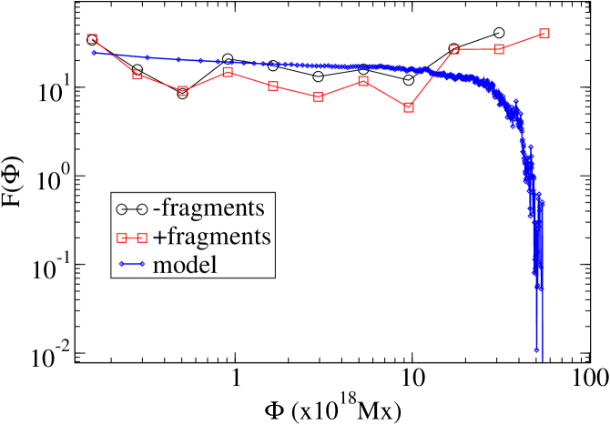
Figure 1: Results demonstrating the scale free network of coronal magnetic flux and comparison with results from numerical simulations of our self-organizing network. For the concentration data $F(\Phi)=constant\times P(\Phi)(\Delta\Phi)\times(\Phi)^{1.7}$, where $P(\Phi)(\Delta\Phi)$ is the normalized number of magnetic concentrations in bins of size $\Delta\Phi=1.55\times 10^{17}$ Mx, obtained by re-analyzing the measurement data originally shown in Figure 5 of Ref. [24]. The model data shown represents the probability distribution, $P(k_{foot})$, for number of loops, $k_{foot}$, connected to a footpoint. This has been rescaled so that one loop, $k_{foot}=1$, equals the minimum threshold of flux, $1.55\times 10^{17}$ Mx. The cutoff at large $\Phi$ in the model data is a finite size effect that can be shifted to larger values or smaller ones by changing the size of the system.

Footpoints aggregate into magnetic “concentrations” on the photosphere. Measuring these concentrations provides a quantitative picture that can be compared with theory. The strongest, and physically largest concentrations are sunspots, which may contain more than $10^{22}$ Mx.[23] The intense magnetic fields in these regions cool the plasma, so they appear dark in the visible spectrum. The smallest resolvable concentrations above the current resolution scale of $\approx 10^{16}$ Mx are “fragments”. Solar physicists have constructed elaborate theories where at each scale a unique physical process is responsible for the dynamics and generation of magnetic concentrations, e.g. a “large scale dynamo” versus a “surface dynamo” etc. These theories predict an exponential distribution for concentration sizes.

2.1 Coronal Fields Form a Scale Free Network

David Hughes and I re-analyzed[17, 18] previously published data sets reporting the distribution of concentration sizes.[24] As shown in Fig. 1, we discovered that the distribution is scale free over the entire range of measurement. The probability to have a concentration with flux $\Phi$, $P(\Phi)\sim\Phi^{-\gamma}$ with $\gamma\approx 1.7$, as indicated by the flat behavior of $F(\phi)$ in Fig. 1. Similar results were found using other data sets.[17]

2.2 The Model

Results from numerical simulations of our network model are also shown in Fig. 1. The only calibration used (which is unavoidable) was to set the minimal unit of flux in the model equal to the flux threshold of the measurement. How did we get such good agreement without solving any of the plasma physics equations?

Considering the long-lived flux tubes as the important coherent structures, we treated the coronal magnetic field as made up of discrete interacting loops embedded in three dimensional space.[16] Each directed loop traces the mid-line of a flux tube, and is anchored to a flat surface at two opposite polarity footpoints. A footpoint locates the center of a magnetic concentration, and is considered to be a point. A collection of these loops and their footpoints gives a distilled representation of the coronal magnetic field structure. Our network model is able to describe the three dimensional geometry of fields that are very complicated or interwoven.

The essential ingredients, which must be included to agree with observations are: injection of small loops, submergence of very small loops, footpoint diffusion, aggregation of footpoints, and reconnection of loops. Observations indicate that all of these physical processes occur in the corona.[20, 21, 24] Loops injected at small length scales are stretched and shrunk as their footpoints diffuse over the surface. Nearby footpoints of the same polarity aggregate, to form magnetic fragments, which can themselves aggregate to form ever larger concentrations of flux. Each loop carries a single unit of flux, and the magnetic field strength at a footpoint is given by the number of loops attached to it. The number of loops that share a given pair of footpoints measures the strength of the link. The link strengths also have a scale-free distribution with a steeper power law than the degree distribution of the nodes, or concentrations. Also, the number of nodes that a given node is connected to by at least one loop is scale-free. Both of these additional claims could also be tested against observations.[17, 18]

Loops can reconnect when they collide, or cross at a point in three dimensional space above the surface. The flux emerging from the positive footpoint of one of the reconnecting loops is then no longer constrained to end up at the other footpoint of the same loop, but may instead go to the negative footpoint of the other loop. This occurs if the rewiring lowers the combined loop length. The loops between the newly paired footpoints then both relax to a semi-circular shape. Reconnection allows footpoints to exchange partners and reshapes the network, but it maintains the degree of each footpoint.

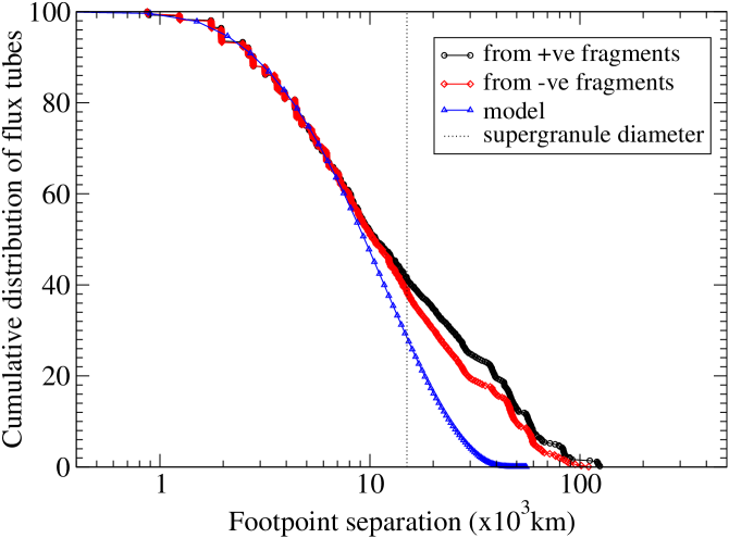
Figure 2: The cumulative percentage of footpoint pairs separated by a distance on the photosphere larger than $d$. The flux tube data corresponds to Figure 6c in Ref. [24]. The model data has been scaled such that one unit of length is equal to 0.5Mm.

If rewiring occurs, one or both loops may need to cross another loop. A single reconnection between a pair of loops can trigger an avalanche of reconnection. Reconnections occur instantaneously compared to the diffusion of footpoints and injection of loops. It may also happen that due to reconnection or footpoint diffusion, very small loops are created. These are removed from the system. Thus the collection of loops is an open system, driven by loop injection with an outflow of very small loops. From any initial condition, the system reaches a steady state where the loops self organize into a scale free network. As shown in Fig. 1 , the number of loops, $k_{foot}$, connected to any footpoint is distributed as a power law

$$P(k_{foot})\sim k_{foot}^{-\gamma}\,\,{\rm\ with\ \ }\gamma=1.75\pm-0.1\quad.$$

2.2.1 Further predictions of the network model

The distribution of distances, $d$, between footpoint pairs attached to the same loop can also be calculated and compared with measurement data as shown in Fig. 2. Indeed, by setting one unit of length in the model equal to $0.5\times 10^{3}$km on the photosphere, good agreement between the model results and observation is obtained up to the supergranule cell size. Deviations above that length scale may be due to several causes: our assumption that the loops are perfectly semi-circular, finite system size effects in the model or observations, or the force free approximation used to calculate the flux tube connectivity from observations of concentrations. Comparing with the observed diffusive behavior of magnetic concentrations[25] allows an additional calibration of time. One unit of time in the model is equal to about 300 seconds on the photosphere. From these three calibrations we are able to determine values for the total solar flux and the “flux turnover time”, which both agree quantitatively with observations. See Ref. [16] for details.

Our model predicts not only nominally universal quantities like various critical exponents characterizing the flux network but also quantities that have typical scales, such as total solar flux, the distribution of footpoint separations, and the flux turnover time in the corona. In order to represent the geometry of the coronal magnetic fields, a three-dimensional model, as discussed here, is required. Whether similar network models can be used to describe other high Reynolds number astrophysical plasmas remains an open question.

3 Seismicity

Despite many efforts, seismicity remains an obscure phenomenon shrouded in vague ideas without benchmarks of testability. At present, no dynamical model can capture, simultaneously, the three most robust statistical features of seismicity: (1) the Gutenberg-Richter (GR) law[26, 27] for the distribution of earthquake magnitudes, and the clustering of activity in (2) space and (3) time. Spatio-temporal correlations include the Omori law[28, 29] for the decay in the rate of aftershocks (see Eq. 4) and the fractal appearance of earthquake epicenters. Note that stochastic processes like the ETAS process[30] require three or more power law distributions to be put in by hand. Since these are the main scaling features (1-3) that we wish to establish a plausible dynamical mechanism for, ETAS models are not regarded by this author as dynamical models of seismicity. To begin with, better methods to characterize seismicity are needed. Here I briefly discuss a network paradigm put forward by Marco Baiesi and myself to this end.[31, 32]

3.1 A Unified Approach to Different Patterns of Seismic Activity

Since seismic rates increase sharply after a large earthquake in the region, events have been classified as aftershocks or main shocks, and the statistics of aftershock sequences have been extensively studied. Usually, aftershocks are collected by counting all events within a predefined space-time window following a main event,[33, 34, 35] These sequences are used e.g. to describe earthquake triggering[36] or predict earthquakes.[37] Obviously, some types of activity, such as swarms, remote triggering,[38] etc. cannot fit into this framework. Perhaps a different description is needed for each pattern of seismic activity. On the other hand, it seems worthwhile to look for a unified perspective to study various patterns of seismic activity within a coherent framework.[39, 40]

What if we do not fix a priori the number of main shocks an event can be an aftershock of? Perhaps an event can be an aftershock of more than one predecessor. On the other hand, all events are not equally correlated to each other. Probably the situation is somewhere in between having one (or zero) correlated predecessors or being strongly correlated to everything that happened before. In fact, a sparse but indefinite property of correlations between events may be ubiquitous to all intermittent spatio-temporal processes with memory.

A sparse network (where each node is an event or earthquake) linking strongly correlated pairs of events stands out as a good starting point for describing seismicity in a unified way. In order to pursue this line of reasoning, we treat all events on the same footing, irrespective of their magnitude, local tectonic features, etc.[40, 41, 42, 43] However, unlike other approaches we do not pre-define any set of space or time windows. The sequence of activity itself selects these. Our method is also unrelated to that of Abe and Suzuki.[44]

3.2 Relations Between Pairs of Events: The Metric

We consider ONLY the relations between earthquakes and NOT the properties of individual events. Only catalogs that are considered complete are examined,[43] and no preferred scales are imposed on the phenomenon. Instead, we invoke a metric to estimate the correlation between any two earthquakes, irrespective of how far apart they are in space and/or time.[31, 32] Consider as a null hypothesis[45] that earthquakes are uncorrelated in time. Pairs of events where the null hypothesis is strongly violated are correlated. The metric measures the extent to which the null hypothesis is wrong.

The specific null hypothesis that we have investigated so far[31, 32] is that earthquakes occur with a distribution of magnitudes given by the GR law, with epicenters located on a fractal of dimension $d_{f}$, randomly in time. Setting $d_{f}=2$ does not change the observed scaling behaviors, nor does varying the GR parameter, $b$.

An earthquake $j$ in the seismic region occurs at time $T_{j}$ at location $R_{j}$. Look backward in time to the appearance of earthquake $i$ of magnitude $m_{i}$ at time $T_{i}$, at location $R_{i}$. How likely is event $i$, given that event $j$ occurred where and when it did? According to the null hypothesis, the number of earthquakes of magnitude within an interval $\Delta m$ of $m_{i}$ that would be expected to have occurred within the time interval $t=T_{j}-T_{i}$ seconds, and within a distance $l=|R_{i}-R_{j}|$ meters, is

$$n_{ij}\equiv(\textit{const})\,t\,l^{d_{f}}\,10^{-bm_{i}}\,\Delta m\quad.$$ (1)

Note that the space-time domain $(t,l)$ appearing in Eq. 1 is self-selected by the particular history of seismic activity in the region and not set by any observer. All earthquake pairs are considered on the same basis according to this metric.

Consider a pair of earthquakes $(i,j)$ where $n_{ij}\ll 1$; so that the expected number of earthquakes according to the null hypothesis is very small. However, event $i$ actually occurred relative to $j$, which, according to the metric, is surprising. A small value $n_{ij}\ll 1$ indicates that the correlation between $j$ and $i$ is very strong, and vice versa. By this argument, the correlation $c_{ij}$ between any two earthquakes $i$ and $j$ can be estimated to be inversely proportional to $n_{ij}$, or

$$c_{ij}=1/n_{ij}\quad.$$ (2)

We measured $c_{ij}$ between all pairs of earthquakes greater than magnitude 3 in the catalog for Southern California from January 1, 1984 to December 31, 2003.[46] The removal of small events assures that the catalog is complete, but otherwise the cutoff magnitude is not important. The distribution of the correlation variables $c_{ij}$ for all pairs ${i,j}$ was observed to be a power law over fourteen orders of magnitude. Since no characteristic values of $c$ appear in this distribution, it doesn’t make sense to talk about distinctly different classes of relationships between pairs. On the other hand, due to the extremely broad distribution, each earthquake $j$ may have exceptional events in its past with much stronger correlation to it than all the others combined. These strongly correlated pairs of events can be marked as linked nodes, and the collection of linked nodes forms a sparse network of disconnected, highly clustered graphs.

3.3 Directed, Weighted Networks of Correlated Earthquakes

A sparse, directed, weighted network is constructed by only linking pairs whose correlation $c$ exceeds a given threshold, $c_{<}$. Each link is directed from the past to the future. For each threshold, $c_{<}$, the error made in deleting links with $c<c_{<}$ can be estimated. For instance, throwing out 99.8% of links gives results accurate to within 1%. This leads to not only massive data reduction with controllable error, but also a renormalized model of seismicity, which extracts the important, correlated degrees of freedom.

Each link contains several variables such as the time between the linked events, the spatial distance between their epicenters, the magnitudes of the earthquakes, and the correlation between the linked pairs. The networks are highly clustered with a universal clustering coefficient $\approx 0.8$ for nodes with small degrees, as well broad, approximately power law in- and out-degree distributions for the nodes.

Consequently, some events have many aftershocks, or outgoing links, while others have one, or zero. Also, some events are aftershocks of many previous events, i.e. they have many incoming links, while others are aftershocks of only one (or zero) events. The data reveal an absence of characteristic values for the number of in or out-going links to an earthquake.[32] For each event $j$ that has at least one incoming link, we define a link weight to each ”parent” earthquake $i$ it is attached to as

$$w_{ij}=\frac{c_{ij}^{\eta}}{\sum_{k}^{\rm in}c_{kj}^{\eta}}\quad,$$ (3)

where the sum is over all earthquakes $k$ with links going into $j$. For instance, an event can be $\frac{1}{2}$ an aftershock of one event, $\frac{1}{3}$ an aftershock of another, and $\frac{1}{6}$ an aftershock of a third. Normally, the parameter $\eta=1$, but it can also be varied without changing the scaling properties of the ensemble of network variables.

3.4 The Omori Law for Earthquakes of All Magnitudes

Fig. 3 shows the rate of aftershocks for the Landers, Hector Mine, and Northridge events. The weights, $w$, of the links made at time $t$ after one of these events are binned into geometrically increasing time intervals. The total weight in each bin is then divided by the temporal width of the bin to obtain a rate of weighted aftershocks per second. The same procedure is applied to each remaining event, not aftershocks of these three. An average is made for the rate of aftershocks linked to events having a magnitude within an interval $\Delta m$ of $m$. Fig. 3 also shows the averaged results for $m=3$ (1871 events), $m=4$ (175 events), $m=5$ (28 events) and $m=5.9$ (4 events).

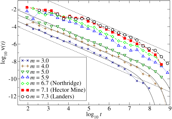
Figure 3: The Omori law for aftershock rates. Rates are measured for aftershocks linked to earthquakes of different magnitudes. For each magnitude, the rate is consistent with the Omori law, Eq. 4. As guides to the eye, dashed lines represent a decay $\sim 1/t$. The dense curves represent the fits obtained by means of Eq. 5 for $m=3$, $m=4$, and $m=5$.

Earthquakes of all magnitudes have aftershocks that decay according to an Omori law,[28, 29]

$$\nu(t)\sim\frac{K}{c+t}\quad,\quad{\rm for}\ t<t_{\rm omori}$$ (4)

where $c$ and $K$ are constant in time, but depend on the magnitude of the earthquake.[29] We find that the Omori law persists up to time $t_{omori}$ that also depends on $m$. The function

$$\nu_{m}(t)\sim t^{-1}e^{-t/t_{\rm omori}}\quad.$$ (5)

was fitted to the data, excluding short times, where the the aftershock rates do not yet scale as $1/t$. The short time deviation from power law behavior is presumably due to saturation of the detection system, which is unable to reliably detect events happening at a fast rate. However, this problem does not occur at later times, where the rates are lower. Some examples of these fits are also shown in Fig. 3 for the intermediate magnitude events. From these fits, a scaling law

$$t_{\rm omori}(m)\simeq 10^{5.25+0.74m}\quad{\rm sec}$$ (6)

was observed for times shorter than the duration of the catalog. It corresponds to $t_{\rm omori}\approx 11$ months for $m=3$, and to $t_{\rm omori}\approx 5$ years for $m=4$. An extrapolation yields $t_{\rm omori}\approx 1400$ years for an event with $m=7.3$ such as the Landers event and $t_{\rm omori}\approx 26,000$ years for the 9.0 Northern Sumatra earthquake causing the 2004 Asian tsunami. These results confirm Kagan’s conjecture that aftershocks can rumble on for centuries.[47] Indeed, with previous measurement techniques it was not possible to test his hypothesis.

4 Acknowledgments

The author thanks David Hughes, Marco Baiesi, and Jörn Davidsen for enthusiastic discussions and their collaborative efforts which contributed to the work discussed here, as well as Peter Grassberger for critical comments on the manuscript. She also thanks her colleagues at the Perimeter Institute, including Fotini Markopoulou and Lee Smolin, for wide ranging conversations.

References

- [1] G. ’t Hooft, L. Susskind, E. Witten, M. Fukugita, L. Randall, L. Smolin, J. Stachel, C. Rovelli, G. Ellis, S. Weinberg and R. Penrose, Nature 433, 7023, 257 (2005).
- [2] L. Smolin, Phil. Trans.: Math., Phys.& Eng. Sci., (Nobel Symposium) 361, [1807] 1081 (2003).
- [3] P. Bak, C. Tang and K. Weisenfeld, Phys. Rev. Lett. 59, 381 (1987).
- [4] U. Frisch, Turbulence (Cambridge University Press, Cambridge, 1995).
- [5] F. S. Labini, M. Montuori and L. Pietronero, Phys. Rep. 293, 62 (1998).
- [6] P. Bak and K. Chen, Phys. Rev. Lett. 86, 4215 (2001).
- [7] P. Bak and M. Paczuski, Physica A 348, 277 (2005).
- [8] F. Markopoulou and L. Smolin, Phys. Rev. D70, 124 029 (2004).
- [9] K. E. Bassler, M. Paczuski and E. Altshuler, Phys. Rev. B64, 224 517 (2001).
- [10] B. Dubrulle, Phys. Rev. Lett. 73, 959 (1994).
- [11] K. Chen and P. Bak, Phys. Rev. E62, 1613 (2000).
- [12] T. Chang, Phys. Plasma 6, 4137 (1999).
- [13] R. Albert and A. -L. Barabási, Rev. Mod. Phys. 74, 47 (2002).
- [14] M. E. J. Newman, SIAM Rev. 45, 167 (2003).
- [15] A. Peel, M. Paczuski and P. Grassberger, in preparation.
- [16] D. Hughes, M. Paczuski, R. O. Dendy, P. Helander and K. G. McClements, Phys. Rev. Lett. 90, 131 101 (2002).
- [17] D. Hughes and M. Paczuski, preprint astro-ph/0309230.
- [18] M. Paczuski and D. Hughes, Physica A 342, 158 (2004).
- [19] For a review see J.B. Zirker, Journey from the Center of the Sun (Princeton University Press, Princeton, 2002).
- [20] E. N. Parker, Astrophys. J. 330, 474 (1988); Sol. Phys. 121, 271 (1989).
- [21] E. N. Parker, Spontaneous Current Sheets in Magnetic Fields (Oxford University Press, New York, 1994).
- [22] E. T. Lu and R. J. Hamilton, Astrophys. J. Lett. 380, L89 (1991).
- [23] One Maxwell (Mx) equals Weber.
- [24] R. Close, C. Parnell, D. MacKay and E. Priest, Sol. Phys. 212, 251 (2003).
- [25] H. J. Hagenaar, C. J. Schrijver, A. M. Title and R. A. Shine, Astrophys. J. 511, 932 (1999).
- [26] B. Gutenberg and C. F. Richter,Seismicity of the Earth, Geol. Soc. Am. Bull. 34, 1 (1941).
- [27] In large seismic regions over long periods of time, the distribution of earthquakes with magnitude , , with .
- [28] F. Omori, J. Coll. Sci. Imp. Univ. Tokyo 7, 111 (1894).
- [29] T. Utsu, Y. Ogata and R. S. Matsu’ura, J. Phys. Earth 43, 1 (1995).
- [30] A. Helmstetter and D. Sornette, Phys. Rev. E66, 061 104 (2002).
- [31] M. Baiesi and M. Paczuski, Phys. Rev. E69, 066 106, (2004).
- [32] M. Baiesi and M. Paczuski, Nonlin. Proc. Geophys. 12, 1 (2005).
- [33] J. Gardner and L. Knopoff, Bull. Seism. Soc. Am. 64, 1363 (1974).
- [34] V. Keilis-Borok, L. Knopoff and I. Rotwain, Nature 283, 259 (1980).
- [35] L. Knopoff, Proc. Natl. Acad. Sci. USA 97, 880 (2000).
- [36] A. Helmstetter, Phys. Rev. Lett., 91, 058 501 (2003).
- [37] Y. Y. Kagan and L. Knopoff, Science 236, 1563 (1987).
- [38] D. P. Hill et al., Science 260, 1617 (1993).
- [39] Y. Y. Kagan, Physica D 77, 160 (1994).
- [40] P. Bak, K. Christensen, L. Danon and T. Scanlon, Phys. Rev. Lett. 88, 178 501 (2002).
- [41] A. Corral, Phys. Rev. E68, 035 102(R) (2003).
- [42] J. Davidsen and C. Goltz, Geophys. Res. Lett. 31, L21 612 (2004).
- [43] J. Davidsen and M. Paczuski, Phys. Rev. Lett. 94, 048 501 (2005).
- [44] S. Abe and N. Suzuki, Europhys. Lett. 65, 581 (2004).
- [45] E. T. Jaynes, Probability Theory: The Logic of Science (Cambridge University Press, Cambridge, 2003).
- [46] The catalog is maintained by the Southern California Earthquake Data Center, and can be downloaded via the Internet at http://www.data.scec.org/ftp/catalogs/SCSN/.
- [47] Y. Y. Kagan in J. R. Minkel, Sci. Am. 286, 25 (2002).