Numerical simulations studies of the convective instability onset in a supercritical fluid

Abstract

Numerical simulation studies in 2D with the addition of noise are reported for the convection of a supercritical fluid, ³He, in a Rayleigh-Bénard cell where the fluid parameters and cell height $L$ are the same as in published laboratory experiments. The noise addition is to accelerate the instability onset after starting the heat flow across the fluid, so as to bring simulations into better agreement with experimental observations. Homogeneous temperature noise and spatial lateral periodic temperature variations in the top plate were programmed into the simulations. A speed-up in the instability onset was obtained, which was most effective through the spatial temperature variations with a period of 2$L$, close to the wavelength of a pair of convections rolls. For a small amplitude of 0.5 $\mu$K, this perturbation gave a semiquantitative agreement with experimental observations. Results for various noise amplitudes are presented and discussed in relation to predictions by El Khouri and Carlès.

I Introduction

In recent papers, convection experiments of supercritical ³He in a Rayleigh-Benard cell with a constant heat current $q$ were reportedKogan:M:2001 ; Meyer:K:2002 . After $q$ is started, the temperature drop $\Delta T(t)$ across this highly compressible fluid layer increases from zero, an evolution accelerated by the “Piston Effect” Onuki:F:1990 ; Zappoli:B:G:LeN:G:B:1990 ; Zappoli:1992 . Assuming that $q$ is larger than a critical heat flux necessary to produce fluid instability, $\Delta T(t)$ passes over a maximum at the time $t=t_{p}$, which indicates that the fluid is convecting and that plumes have reached the top plate. Then truncated or damped oscillations, the latter with a period $t_{\rm osc}$, are observed under certain conditions before steady-state conditions for convection are reached, as described in refs.Kogan:M:2001 ; Meyer:K:2002 . The scenario of the damped oscillations, and the role of the “piston effect” has been described in detail in refs.Furukawa:O:2002 and Amiroudine:Z:2003 and will not be repeated here. The height of the layer in the RB cell was $L$ = 0.106 cm and the aspect ratio $\Gamma$=57. The ³He convection experiments along the critical isochore extended over a range of reduced temperatures between 5$\times 10^{-4}\leq\epsilon\leq$ 0.2, where $\epsilon=(T-T_{c})/T_{c}$ with $T_{c}$ = 3.318 K, the critical temperature. The truncated - or damped oscillations were observed for $\epsilon\geq$ 0.009 and over this range the fluid compressibility varies by a factor of about 30.

The scaled representation of the characteristic times $t_{\rm osc}$ and $t_{\rm p}$ versus the Rayleigh number, and the comparison with the results from simulations has been described in ref.Furukawa:M:O:K:2003 . Good agreement for the period $t_{\rm osc}$was reported. However a systematic discrepancy for the times $t_{\rm p}$ shows that in the simulations the development of convection is retarded compared to the experiments. This effect increases with decreasing values of $[Ra^{\rm corr}-Ra_{c}]$, where $Ra^{\rm corr}$ is the Rayleigh number corrected for the adiabatic temperature gradient as defined in refs.Kogan:M:2001 ; Meyer:K:2002 and $Ra_{c}$ is the critical Rayleigh number for the experimental conditions, 1708. This is shown in Fig.1 of ref.Furukawa:M:O:K:2003 , in particular in Fig.1b) for $\epsilon$ = 0.2 and $q$ = 2.16$\times 10^{-7}$ W/cm² ($[Ra^{\rm corr}-Ra_{c}]$ = 635), where an experimental run is compared with simulations for the same parameters. Here clearly the profile $\Delta T(t)$ from the simulations shows the smooth rise until the steady-state value, $\Delta T=qL/\lambda$ = 95 $\mu$K has been reached, where $\lambda$ is the thermal conductivity. Only at t $\approx$ 90 s. does convection develop, as shown by a sudden decrease of $\Delta T(t)$. By contrast, the experimental profile shows a much earlier development of convection. Fig.1 of ref.Furukawa:M:O:K:2003 is representative for the observations at low values of $[Ra^{\rm corr}-Ra_{c}]$. At high values, both experiment and simulations show the convection development to take place at comparable times, as indicated in Fig.5b) of ref.Furukawa:M:O:K:2003 , and specifically in Fig.2 a) of ref.Amiroudine:Z:2003 , where $[Ra^{\rm corr}-Ra_{c}]$ =4.1$\times 10^{5}$. It is the purpose of this report to investigate the origin of this discrepancy by further simulation studies.

II Convection onset calculations, simulations and comparison with experiments

El Khouri and CarlèsElKhouri:C:2002 studied theoretically the stability limit of a supercritical fluid in a RB cell, when subjected to a heat current $q$ started at the time $t$ = 0. Their fluid was also ³He at the critical density, and the same parameters as in ref.Kogan:M:2001 were used. They calculated the time $t_{\rm instab}$ and also the corresponding $\Delta T(t_{\rm instab})$ for the onset of fluid instability and they determined the modes and the wave vectors of the perturbations for different scenarios of $q$ and $\epsilon$. For $t>t_{\rm instab}$ inhomogeneities in the RB cell and noise within the fluid will produce perturbations which will grow, from which the convection will develop. An indication of the growth of convection is a deviation of the $\Delta T(t)$ profile in the experiments or in the simulations from the calculated curve for the stable fluid (see for instance Eq.3.3 of refFurukawa:O:2002 ). It is readily seen from simulation profiles such as Fig.1a) and b) in ref.Furukawa:O:2002 that the deviation becomes significant for $t$ only slightly below $t_{\rm p}$ - the maximum of $\Delta T(t)$. In simulations, the effective start of convection can also be seen from snapshots in 2D of the fluid temperature contour lines at various times, as shown in Fig. 5 of ref.Chiwata:O:2001 .

P.Carlès Carles:2003 has argued that the reason for the discrepancy for the time $t_{\rm p}$ between experiment and simulation is that in the former, the physical system has noise and inhomogeneities which cause the perturbations beyond $t_{\rm instab}$ to grow into the developed convection. By contrast simulations have a much smaller noise. Therefore in the simulations the perturbations take a longer time to grow than in the physical system, leading to a larger $t_{\rm p}$ than observed. Carlès’ comment led us to try as a first step imposing a thermal random noise on the top plate of the RB cell, which was to simulate fluctuations in the upper plate temperature control of the laboratory experiment. The temperature of the plate was assumed to be uniform, because of the large thermal diffusivity $D_{T}\approx 2\times 10^{4}$ cm²/s. of the copper plate in the experiments. Accordingly simulations were carried out by the numerical method described in ref.Furukawa:O:2002 with a homogeneous time-dependent temperature random fluctuation of given rms amplitude imposed on the upper plate. This implementation consisted in adding or subtracting randomly temperature spikes $T_{t}$ at the time $t$ with a programmed rms amplitude at steps separated by 0.02 s. This interval is much larger than the estimated relaxation time of the top plate over a distance $2L$, approximately the wavelength of convection roll pair. Values of the variance A = $\sqrt{<(T_{t}-<T_{t}>)^{2}>}$ were chosen between 0 and 40 $\mu$K. The range of the A values was taken well beyond the estimated fluctuation rms amplitude during the experimentsKogan:M:2001 of $\approx 1\mu K/\sqrt{Hz}$. Three representative curves with 0, 3 and 40 $\mu$K are shown in Fig.1a) by dashed lines for $\epsilon$ = 0.2 for $q$= 2.16$\times 10^{-7}$ W/cm², $L$ = 0.106cm and $\Gamma$ = 5.1. For this value of $q$, the calculation by El Khouri and Carlès ElKhouri:C:2004 give $t_{\rm instab}$ = 6.3 s and $\Delta T(t_{\rm instab})$ = 75 $\mu$K. In the simulation without imposed noise, the start of convection has therefore been considerably delayed relative to $t_{\rm instab}$. The injection of random noise has a significant effect in developing convection at an earlier time. In Fig.1a) the three curves are also compared with the experimental one, shown by a solid line. Here we have not incorporated into the simulations the delay affecting the experimental temperature recording, so that they could be intercompared more readily, and also with predictionsElKhouri:C:2004 However this operation will be presented in Fig.4. Further simulations with added random noise were carried out for $\epsilon$ = 0.2 and 0.05 where the $\Delta T(t)$ time profiles are not shown here.

Fig.2a) shows a plot of the time of the developed convection, represented by $t_{\rm p}$, versus the random rms amplitude A for three series of simulations, all taken for a cell with $\Gamma$ = 5.1. They are a) and b) $\epsilon$ = 0.2, $q$ = 2.16 and 3.89$\times 10^{-7}$W/cm², and c) $\epsilon$ = 0.05, $q$ = 60 nW/cm², ([$Ra^{\rm corr}-Ra_{c}$] = 635, 1740 and 4200). The simulation results, shown by solid circles, are compared with the experimentally observed $t_{\rm p}$ shown by horizontally dot-dashed lines. It can be clearly seen that noise imposition, which creates a vertical disturbance across the fluid layer, reduces the time of convection development. While the decrease of $t_{\rm p}$ is strong for small values of A, it saturates at a certain level of noise amplitude. The gap between simulations and experiment increases with a decrease of [$Ra^{\rm corr}-Ra_{c}$], namely as the fluid stability point is approached. A “critical slowing down” is seen in the effectiveness of the perturbations in triggering the instability. Hence this mode of noise introduction fails, because its amplitude is limited to the vertical z direction and it evidently couples only weakly into the convective motion.

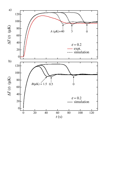
Figure 1: a) the temperature profile $\Delta T(t)$ from experiments (solid line with noise) and from several simulations (dashed lines) at $\epsilon$ = 0.2, $q$= 2.16$\times 10^{-7}$ W/cm². In the simulations, $\Gamma$=5 and uniform temperature noise has been imposed on the top plate with variance $A(\mu K)$ = 0, 3 and 40, as described in the text. b) Temperature profile $\Delta T(t)$ from several simulations at $\epsilon$ = 0.2, $q$= 2.16$\times 10^{-7}$ W/cm², $\Gamma$ = 8 and imposed lateral periodic, time independent temperature variations on the top plate with period $2L$ and amplitude $B(\mu K)$ = 0, 0.5 and 1.5.

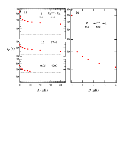
Figure 2: a) The time for effective development of convection, characterized by $t_{\rm p}$, versus $A$ (homogeneous temperature noise imposed on the top plate). The horizontal dot-dashed lines indicate the observed $t_{\rm p}$, corrected for instrumental recording delay. b) The time for effective development of the convection, labeled by $t_{\rm p}$ versus $B$ (lateral time-independent periodic temperature variations). The horizontal dashed line indicates $t_{\rm p}$ as obtained by experiment, corrected as before.

In parallel with the present experiments, S. AmiroudineAmiroudine:2004 also carried out a systematic study of simulations on supercritical ³He in a RB cell for several values of $\epsilon$ and $q$. He used a numerical scheme based on the exact Navier Stokes equation as described in ref.Amiroudine:Z:2003 . The resulting profiles $\Delta T(t)$ could be compared with those from experiments done under nearly the same conditions. In his simulations, homogeneous temperature random noise was again imposed on the top plate. The shift in $t_{\rm p}$ showed less systematic trends than in the results described in this report. However for the same values of $\epsilon$ and $q$ as those reported above, and at zero noise, the $t_{\rm p}$ values tended to be somewhat smaller than in the results of Fig 2a).

Here we mention that the onset of convection in the simulations is further influenced by the aspect ratio $\Gamma$. The simulations described above, but without noise, were carried out in a cell $\Gamma$ = 5.1 having periodic lateral boundaries. Further simulations with zero noise for $\epsilon$ = 0.2 with $\Gamma$ = 8.0, 10.2, 20.5 and 41.0 were carried out, and showed a decrease of the convection development time from $\approx$ 90 s, tending to a constant value of $\approx$ 60 s. above $\Gamma$ = 20. This shift in the onset of instability is due to the decreased finite size effect which the rising plumes experience with increasing $\Gamma$, in spite of the periodic boundary conditions. This can be seen by comparing the curves labeled “O” in Figs 1a and 1b with $\Gamma$ = 5 and 8 respectively.

The next step in our attempts, stimulated by communications with P. Carlès, was introducing perturbations into the simulations via some time-independent lateral variation proportional to sin (2$\pi x/P$) where $P$ is the period. We opted to introduce again a temperature variation in the top plate with an amplitude B (in $\mu$K) and period $P$=2$L$, nearly the same as the wavelength of a pair of convection rolls. The temperature of the bottom plate was kept homogeneous. This “Gedanken Experiment” implies that the material of the top plate permitted a temperature inhomogeneity, which of course is not realized in the experiment. However a small lateral temperature excursion can trigger the same kind of non-homogeneous perturbations as those which, in the real experiment, provoke the onset of convection. One possible origin of such perturbations, besides thermal noise, could be the roughness of the plates or their slight deviation from parallelism. Such geometrical defects could of course not be implemented in the numerical simulations with the meshsize used, which is why we elected to force a small temperature perturbation instead, with similar effects on the onset. As a control experiment, we also made a simulation with $P=L$.

Fig 1b) shows representative profiles $\Delta T(t)$ for the parameters $\epsilon$ = 0.2 and $q$= 2.16$\times 10^{-7}$ W/cm² and with B = 0, 0.5 and 1.5 $\mu$K, and for $\Gamma$=8. As B is increased from zero, there is a large decrease in the time for convection development, represented by $t_{\rm p}$, which is plotted versus B in Fig 2b). The horizontal dashed line shows the $t_{\rm p}$ from the experiment, and this plot is to be compared with Fig. 2a). For an inhomogeneity amplitude of only B= 0.5$\mu$K, $t_{\rm p}$ is nearly the same for simulations and experiment. By contrast, simulations with B=2$\mu$K and $P$=$L$ (not presented here) show no difference from those with B=0. Hence the nucleation of the convection is accelerated if the period is in approximate resonance with the wavelength of a convection roll pair. The values of steady-state $\Delta T$ and $t_{\rm osc}$ are only marginally affected by the noise.

We note from Fig.1b) that the simulation curve calculated for B = 0 shows the fluid not convecting until $\approx$ 70 s. For the curves with B= 0.5 $\mu$K., the start of deviations from the stable fluid curve cannot be estimated well from Fig.1b) but is readily obtained from the data files, which tabulate $\Delta T(t)$ to within 1 nK. For B = 0.5 $\mu$K, systematic deviations $\delta\Delta T(t,B)\equiv[\Delta T(t$,B=0) - $\Delta T(t$,B)] increase rapidly from 1 nK for $t>$8 s (where $\Delta T\approx$85 $\mu$K), a value comparable with the predicted $t_{\rm instab}$= 6.3 s., $\Delta T(t_{\rm instab})$ = 75$\mu$KElKhouri:C:2004 . However a comparison with predictions becomes more uncertain as B is increased and no longer negligible compared with the steady-state $\Delta T$. Then it is expected that the base Piston-Effect heat flow will become itself influenced by the perturbations. In that case the stability analysis in ElKhouri:C:2004 becomes irrelevant, since the base flow, the stability of which is analysed, has been significantly modified by the perturbations. We also note that the time interval $\delta t\equiv[t_{\rm p}-t_{\rm instab}$] between the first sign of instability ($\delta\Delta T>0$) and $t_{\rm p}$ is $\approx$ 20 s, and roughly independent of B. This represents approximately the period taken by the convection to develop and for the plumes to reach the top plate boundary.

In Fig.3, we present a series of 2D “snapshots” at various times for the simulation with B = 0.5$\mu$K, showing the temperature contour lines (in color) for the RB cell. The “warm” side is shown by red, $T(t,z=0)$ and the “cold” side by mauve, $T(z=L)$ = const. At $t$= 8 s. the fluid instability has just started near the top of the layer, while near the bottom the

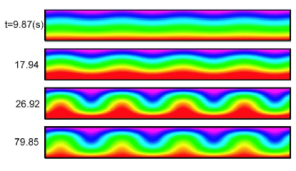
Figure 3: Snapshots in 2D for the RB cell with an aspect ratio of 8, of simulations with B = 0.5 $\mu K$ at various times $t$ after starting the heat current $q$. The temperature contour lines and their evolution are described in the text. At the time $t$ = 9.9s, the fluid instability has just started near the top.

temperature contour lines are still horizontal. At t = 27 s., where the peak of $\Delta T(t)$ at $z=L$ has been reached, the warm plumes have reached the top plate, and the “cold” piston effect is about to start, causing the bulk fluid temperature to drop and $\Delta T(t)$ to decrease. The transient process continues with damped oscillations of $\Delta T(t)$. Steady state convection is reached at t= 80s, with a pair of convection rolls having a wavelength of $\approx$ 2$L$, as expected.

In Fig.4 we show the profiles $\Delta T(t)$ from the experiment and from the simulations with a periodic perturbation amplitude B = 0.5 $\mu$K. For an optimal comparison, the delay affecting the experimental temperature recording was incorporated into the simulation curve. For this, the delay function with the instrumental time constant $\tau$ = 1.3 s. Kogan:M:2001 was folded into the simulation curve by a convolution method. This operation retards the initial rise of the temperature drop by the order of 2-3 seconds, and brings both experiment and simulations into fair agreement in the regime where the fluid is stable. The time $t_{\rm p}$ for the maximum is now closely the same for both experiments and simulations. However beyond the predicted instability time $t_{\rm instab}$= 6.3 s., the experimental curve starts to deviate more rapidly with time than do the numerical simulations from the calculated curve for the fluid in the stable regime. As discussed previouslyMeyer:K:2002 , for these parameters of $\epsilon$ and $q$ the experiment does not show damped oscillations, which are observed for higher values of $q$. In the steady-state, the agreement is very good.

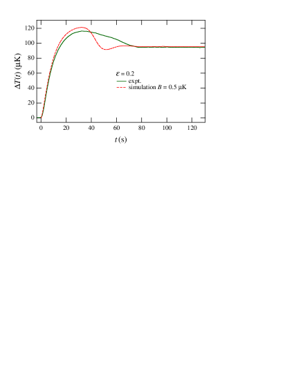
Figure 4: Comparison of the profile $\Delta T(t)$ from experiment and from simulations with B = 0.5 $\mu K$ . To make the comparison realistic, the simulations have been convoluted with the same “instrumental” delay time $\tau$ =1.3 s. which has influenced the shape of the experimental curve.

Our goal has been to show that injecting a small temperature perturbation into the top plate, produces for the simulations an earlier start in the convective instability, which becomes consistent with experimental observations. For this, we have limited ourselves to an example at a low value of $[Ra^{\rm corr}-Ra_{c}]$, where the delay has been particularly large with respect to the experiment.

III Summary and Conclusion

We have presented a comparison of numerical simulations with experimental data investigating the transient to steady convection after the start of a heat current through a supercritical ³He layer in a RB cell. Here the temperature drop $\Delta T(t)$ across the fluid layer versus time $t$ was studied. The aim was to understand and to reduce the discrepancy between experiment and simulations in the time of the convection development, as detected by $\Delta T(t)$. Simulations for one set of fluid parameters (where the largest discrepancy had been observed) are reported with imposed temperature variations on the top plate. Satisfactory results were obtained for spatial lateral temperature variations with an amplitude of 0.5 $\mu$K and a period approximately equal to that of the wavelength of a convection roll pair. As the perturbation amplitude is further increased, the development of convection occurs earlier than the observed one.

IV Acknowledgment

The authors are greatly indebted to P. Carlès for stimulating correspondence and suggestions, to F. Zhong for help with figures formatting and the convolution program in Fig.3 and to R.P. Behringer and P. Carles for useful comments on the manuscript. The interaction with S. Amiroudine, who conducted numerical simulation in parallel with present investigations is greatly appreciated. The work is supported by the NASA grant NAG3-1838 and by the Japan Space Forum H12-264.

References

- (1) A.B. Kogan and H. Meyer, Phys. Rev. E 63, 056310 (2001).
- (2) H. Meyer and A.B. Kogan, Phys. Rev. E 66,056310 (2002).
- (3) A. Onuki and R.A. Ferrell, Physica A 164, 245 (1990).
- (4) B. Zappoli, D. Bailly, Y. Garrabos, B. le Neindre, P. Guenoun and D. Beysens, Phys. Rev. A 41, 2264 (1990).
- (5) B. Zappoli, Phys. of Fluids 4, 1040 (1992), B. Zappoli and P. Carles, Eur. J. Mech. B/Fluids 14. 41, (1995)
- (6) A. Furukawa and A. Onuki Phys. Rev. E 66, 016302 (2002).
- (7) S. Amiroudine and B. Zappoli, Phys. Rev. Lett. 90, 105303 (2003).
- (8) A. Furukawa, H. Meyer, A. Onuki and A.B. Kogan, Phys. Rev. E 68, 056309 (2003)]
- (9) L. El Khouri and P. Carlès, Phys. Rev. E 66, 066309 (2002).
- (10) Y. Chiwata and A. Onuki, Phys. Rev. Lett. 87, 144301 (2001).
- (11) P. Carlès, private communication.
- (12) L. El Khouri and P. Carlès, Private communication.
- (13) S. Amiroudine, private communication.