Transonic instabilities in accretion disks
Abstract
In two previous publications [1] ; [2] , we have demonstrated that stationary rotation of magnetized plasma about a compact central object permits an enormous number of different MHD instabilities, with the well-known magneto-rotational instability [3] ; [4] ; [5] as just one of them. We here concentrate on the new instabilities found that are driven by transonic transitions of the poloidal flow. A particularly promising class of instabilities, from the point of view of MHD turbulence in accretion disks, is the class of trans-slow Alfvén continuum modes, that occur when the poloidal flow exceeds a critical value of the slow magnetosonic speed. When this happens, virtually every magnetic/flow surface of the disk becomes unstable with respect to highly localized modes of the continuous spectrum. The mode structures rotate, in turn, about the rotating disk. These structures lock and become explosively unstable when the mass of the central object is increased beyond a certain critical value. Their growth rates then become huge, of the order of the Alfvén transit time. These instabilities appear to have all requisite properties to facilitate accretion flows across magnetic surfaces and jet formation.
I Introduction
In Fig. 1, a Magnetized Accretion-Ejection Structure is shown which illustrates the problem we wish to address in this paper, viz.: How does an accretion flow about a compact object first crosses the magnetic configuration and then turns the corner with respect to the accretion disk to produce jets? In ideal MHD, plasma and magnetic field stay together (frozen in field), so that a sizeable resistivity is needed for the flow to detach from the magnetic field. This involves anomalous dissipation. Hence, the basic problem is to find relevant local instabilities producing the necessary MHD turbulence.
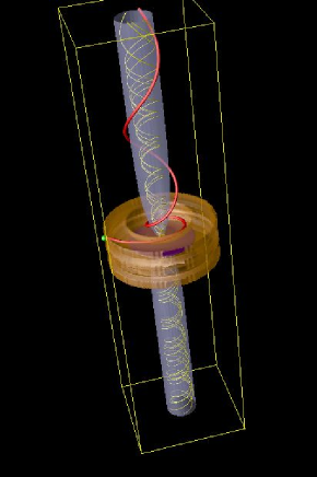

Our model is shown in Fig. 2: An axisymmetric configuration of nested magneticflow surfaces with magnetic field indicated by the vectorial Alfvén speed and velocity , having both toroidal and poloidal components, surrounds a compact object of mass in the origin. Note that the usual tokamak configuration is obtained for , whereas accretion disk geometries may have flat (thin disk) as well as round (thick disk) poloidal cross-sections. [9] This model considers laboratory and astrophysical toroidal plasmas on an equal footing by exploiting the scale independence [10] of the MHD equations.

In order to obtain a stationary equilibrium situation, we assume that the accretion flow speed is much smaller than both rotation speeds of the disk. We then need to determine the stationary equilibrium flows (Sec. 2) and, next, the local instabilities driven by the transonic flow (Sec.3). We analyze this problem from two angles:
(a) Asymptotic analysis for small inverse aspect ratio ();
(b) Large-scale exact numerical computations of the equilibria and instabilities.
These will be discussed in reverse order since the numerical results suggest the relevant approximations that may be made.
A difficulty encountered is that transonic transitions upset the standard equilibrium–stability split. We will discuss this in Sec. 2 under the heading of transonic enigma.
The gravitational parameter exploited here is defined as follows:
| (1) |
This parameter measures the deviation from Keplerian flow (for which ).
II Transonic equilibrium flows
We exploit a variational principle for the stationary axisymmetric equilibria determining the poloidal flux and the poloidal Alfvén Mach number squared This involves five arbitrary scaled flux functions :
| (2) | |||||
| (3) | |||||
| (4) | |||||
| (5) | |||||
| (6) |
which have to be fixed by whatever observational evidence is available. Note that the flux function (6) has been renamed (instead of the usual ) to eliminate the confusion derived from the frequent occurrence of the misnomer ‘specific angular momentum’ in the astrophysics literature (see references in Ref. [2], ). This is important since one of the essential problems in accretion disk dynamics is precisely the transport of angular momentum.
The stationary states are then determined by minimization of the following Lagrangian:
| (7) |
where are simple algebraic expressions. The Euler equations provide the solutions and of the core variables. [ A generalization of this variational principle to two-fluid plasmas is given in Ref. [11], . ]
The transonic enigma mentioned above is due to the fact that the flows suddenly change character from elliptic to hyperbolic at the transonic transitions. As a result, standard (tokamak) equilibrium solvers diverge in the hyperbolic regimes! We circumvent this problem by calculating in elliptic regimes beyond the first hyperbolic one. Obviously, the payoff is that we cannot approach the transonic transitions but have to infer what has happened there from the changes in the dynamics found in the ‘transonic’ elliptic regimes.
The pleasing side of the transonic enigma is that the time-dependence of the linear waves and the spatial dependence of the nonlinear stationary states are intimately related. This is seen by comparing the wave spectra, which cluster at the slow, Alfvén, and fast continuum frequencies , , for highly localized modes (Fig. 3),

and the corresponding slow, Alfvén, and fast hyperbolic flow regimes delimited by critical values of the square of the poloidal Alfvén Mach number (Fig. 4):

By means of the transonic equilibrium solver FINESSE (described in Ref. [12], ) typical equilibria in the first trans-slow elliptic regime have been computed for tokamak and accretion disk (Figs. 5, and 6) for a representative choice of the flux function parameters:


Note that the accretion disk equilibrium, in contrast to the tokamak, has the density peaking on the outside to produce overall equilibrium on the fluxflow surfaces with respect to the gravitational pull of the compact object in the center. For the sake of the spectral calculations (Sec. 3), the two equilibria have been chosen such that the safety factor is a monotonically increasing function.
III Local transonic instabilities
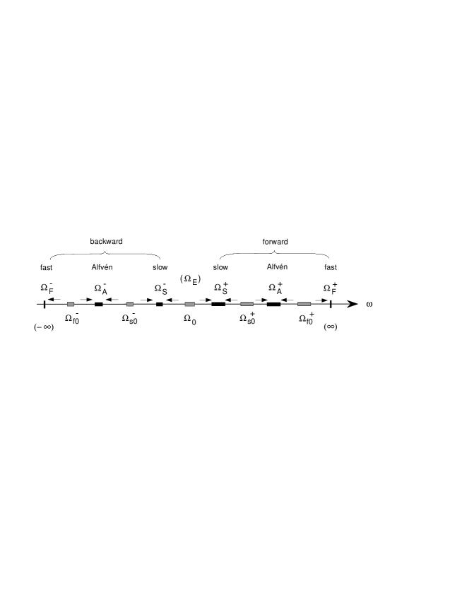
With equilibrium flows, the overall spectral structure of MHD waves and instabilities is determined by the split in forward and backward waves so that the local waves cluster at the Doppler shifted continuous spectra:
| (8) |
These are embedded in a monotonic spectral structure for 1D equilibria, as shown in Fig. 7. A long-standing puzzle about the nature of the singular frequencies () has been clarified in Ref. [13], : In the Eulerian description, these frequencies give rise to the Eulerian entropy continua (), not perturbing the pressure, velocity, and magnetic field, and, hence, absent in the Lagrangian description.
To solve for the local transonic instabilities, we exploit the Frieman-Rotenberg equation,
| (9) |
The linear operator is no longer self-adjoint, so that overstable modes occur, in particular in 2D axisymmetric equilibria through coupling of the poloidal modes .
In order to solve for the transonic continuum modes we exploit localization on separate magnetic / flow surfaces,
| (10) |
This gives rise to an eigenvalue problem for each surface,
| (11) |
where the matrices are defined by
| (14) | |||||
| (17) |
and the Doppler shifted frequency in a frame rotating with .
The overall result of the analysis of this eigenvalue problem (11) is that the continuum modes are always unstable in the trans-slow () flow regime! This is due to the poloidal derivatives indicated by the terms multiplied with factors . The instability mechanism involves coupling of the Alfvén and slow continuum modes.
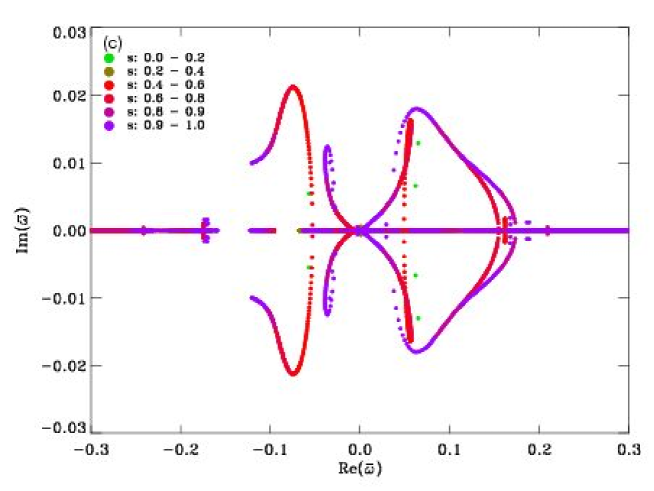
Fig. 8 shows the full complex spectrum of trans-slow Alfvén continuum ‘eigenvalues’ for a Tokamak () equilibrium with the radial coordinate as a parameter. The colors indicate on which magneticflow surface the modes are localized. The modes rotate clockwise for Re and anti-clockwise for Re, and have growth rates of the order of a few percent of the inverse Alfvén transit time.
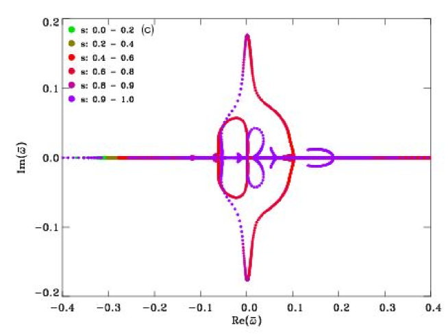
The counterpart for an accretion disk () equilibrium is shown in Fig. 9. Now the rotating continuum modes lock to give purely exponential growing modes (Re) over a sizeable range of magneticflow surfaces. Their growth rates are huge, in the order of ten to twenty percent of the inverse Alfvén transit time! Consequently, these modes have enough time to saturate during a finite number of revolutions of the plasma.
Analysis of the dispersion equation by small inverse aspect ratio expansion () is suggested by the numerical results, which exhibit dominant coupling of the six Alfvén and slow continuum modes , , around the degeneracies at the rational surfaces . This analysis confirms that the trans-slow Alfvénic continuum modes are unstable at, or close to, the rational surfaces for all toroidal mode numbers .
For a very massive central object (), the growth rate in the limit becomes
| (18) |
which is far in excess of the Alfvén frequency.
Since these modes are localized both radially (because of the continuous spectrum) and in the angle (and ) they are perfectly suitable to produce the turbulence that is needed along the accretion flow at the inner edge of the accretion disk with respect to the central object to detach the flow from the magnetic field.
IV Conclusions
(1) In the presence of poloidal rotation, the singular structure of the MHD continua transfers to the equilibrium, so that linear waves and non-linear stationary equilibrium flows are no longer separate issues.
(2) Complete spectra of waves and instabilities have been computed for tokamaks and accretion disks with transonic flows exploiting our new computational tools FINESSE (for equilibria) and PHOENIX (for stability).
(3) We have found a large class of instabilities of the continuous spectra of transonic axisymmetric equilibria for .
(4) These instabilities may cause strong MHD turbulence and associated anomalous dissipation, breaking the co-moving constraint of plasma and magnetic field and facilitating both accretion and ejection of jets from accretion disks.
Acknowledgements
This work was performed as part of the research program of the Euratom-FOM Association Agreement, with support from the Netherlands Science Organization (NWO). The National Computing Facilities (NCF) is acknowledged for providing computer facilities.
References
- (1) R. Keppens, F. Casse, J.P. Goedbloed, “Waves and instabilities in accretion disks: Magnetohydrodynamic spectroscopic analysis”, Astrophys. J. 569, L121–L126 (2002).
- (2) J.P. Goedbloed, A.J.C. Beliën, B. van der Holst, R. Keppens, “Unstable continuous spectra of transonic axisymmetric plasmas”, Phys. Plasmas 11, 28–54 (2004).
- (3) E.P. Velikhov, “Stability of an ideally conducting liquid flowing between cylinders rotating in a magnetic field”, Soviet Phys.–JETP Lett. 36, 995 (1959).
- (4) S. Chandrasekhar, “The stability of non-dissipative Couette folow in hydromagnetics”, Proc. Nat. Acad. Sci. USA 46, 253 (1960).
- (5) S.A. Balbus and J.F. Hawley, “A powerful local shear instability in weakly magnetized disks. I. Linear analysis”, Astrophysical Journal 376, 214 (1991).
-
(6)
G. Tóth,“A general code for modeling MHD flows on parallel computers: Versatile Advection Code”, Astrophys. Lett. & Comm. 34, 245 (1996).
http://www.phys.uu.nl/~toth/ - (7) F. Casse and R. Keppens, “Radiatively inefficient MHD accretion-ejection structures”, Astrophys. J. 601, 90 (2004).
- (8) F. Casse and R. Keppens, “Magnetized accretion-ejection structures: 2.5 D MHD simulations of continuous ideal jet launching from resistive accretion disks”, Astrophys. J. 581, 988 (2002).
- (9) J. Frank, A. King, and D. Raine, Accretion Power in Astrophysics, 3rd edition (Cambridge University Press, Cambridge, 2002).
-
(10)
J.P. Goedbloed and S. Poedts, Principles of Magnetohydrodynamics, with Applications to Laboratory and Astrophysical Plasmas (Cambridge University Press, Cambridge, 2004).
http://titles.cambridge.org/catalogue.asp?isbn=0521626072 - (11) J.P. Goedbloed, “Variational principles for stationary one- and two-fluid equilibria of axisymmetric laboratory and astrophysical plasmas”, Phys. Plasmas 11, to appear (December 2004).
- (12) A.J.C. Beliën, M.A. Botchev, J.P. Goedbloed, B. van der Holst, R. Keppens, “FINESSE: Axisymmetric MHD equilibria with flow”, J. Comp. Phys. 182, 91–117 (2002).
- (13) J.P. Goedbloed, A.J.C. Beliën, B. van der Holst, R. Keppens, “No additional flow continua in magnetohydrodynamics”, Phys. Plasmas 11, 4332–4340 (2004).