Marginal Confinement in Tokamaks by Inductive Electric Field

Abstract

Here diffusion and Ware pinch are analyzed as opposed effects for plasma confinement, when instabilities are not considered. In this work it is studied the equilibrium inductive electric field where both effects annul each other in the sense that the average normal velocity is zero, that is, marginal velocity confinement is reached. The critical electric field defined in that way is studied for different values of elliptic elongation, Shafranov shift and triangularity. A short complementary analysis is also performed of the variation of the poloidal magnetic field along a magnetic line. Magnetohydrodynamic transport theory in the collisional regime is used as in recent publications. Axisymmetric and up-down symmetry are assumed.

I Introduction

The H-mode is characterized by the suppression of anomalous transport in tokamaks, because of low plasma turbulence induces by internal barriers[1-3]. As result neoclassical transport calculations becomes very important in this mode. Diffusion in the collisional regime depends of the pressure gradient at the 95% surface adjacent to the scrape of layer or SOL, as well as the inductive electric field $E_{\varphi}$. The diffusion due to the gradient pressure is opposed to Ware the pinch effect due to $E_{\varphi}$.
In previous papers was shown that neoclassical diffusion can be treated with great simplicity in the case of arbitrary plasma configuration, using a new kind of tokamaks coordinates described there[4-6]. However, suitable direct numerical calculations for different values of elongation, Shafranov shift and triangularity have not been presented until now. Some previous results on this theme using these coordinates are incomplete, and they are not using the right parameters for the tokamaks in operation at present.
Here calculations are presented in a different way, since we look for the values of $E_{\varphi}$ in the marginal velocity confinement, that is, when the average velocity on 95 % surface is zero the results corresponding to marginal confinement flux, that is, the transition from the outgoing to ingoing flux, could be more interested, but much more difficult to calculate and a suitable and simple treatment describing this process for any plasma configuration seem that they have not been publishing until now.
In the calculations now presented there are first a suitable normalization procedure absent in previous calculations as well as an adequate selection of tokamak parameters. The normalization used here allows us to get results, which can be useful for a diversity of different tokamak plasma configurations, with different values of ellipticity, Shafranov shift and triangularity.

II Theoretical Treatment

The collisonal transport treatment presented in previous paper for toroidal axisymmetric plasmas can be written in a more convenient way using dimensionless integrals and variables, as

$$\tilde{v}=\frac{<v>}{-\frac{{\eta}_{\bot}}{B^{2}_{\varphi 1}}\ (\frac{\partial p}{\partial\sigma})_{1}}=\frac{1}{\hat{I}_{0}}[\frac{\hat{I}_{2}}{(R_{1}/R_{c})^{2}}+\frac{{\eta}_{\|}}{{\eta}_{\bot}{\gamma}^{2}_{1}(R_{1}/R_{c})^{2}}(\hat{I}_{3}-\frac{\hat{I}^{2}_{1}}{\hat{I}_{4}})]-\frac{\tilde{E}_{\varphi 1}}{\gamma_{1}\hat{I}_{0}}(\hat{I}_{7}-\frac{\hat{I}_{1}\hat{I}_{6}}{\hat{I}_{4}}+{\gamma}^{2}_{1}\hat{I}_{5})\ \ ,$$ (1)

where $\tilde{v}$ is the dimensionless normal velocity derived from the velocity $<v>$ along the magnetic surface normal, and $\tilde{E}_{\varphi 1}$ is a dimensionless electric field defined as

$$\tilde{E}_{\varphi}=\frac{{E}_{\varphi}}{-\frac{{\eta}_{\bot}}{B_{\varphi 1}}\ (\frac{\partial p}{\partial\sigma})_{1}}\ \ .$$ (2)

Her $R_{1}$, $B_{\varphi 1}$, $B_{p1}$, ${E}_{\varphi 1}$ and $(\frac{\partial p}{\partial\sigma})_{1}$ are respectively the major radius, toroidal and poloidal magnetic field, inductive electric field and pressure gradient at the mid-plane external point $A_{0}$ of the magnetic cross section. The plasma resistivity are ${\eta}_{\bot}$ and ${\eta}_{\|}$ in the directions perpendicular and parallel to the magnetic field lines and $R_{c}$ is the minor axis radius. The dimensionless quantity ${\gamma}_{1}$ is the ratio $\gamma_{1}=B_{p1}/B_{\varphi 1}$ between poloidal and toroidal magnetic field at point $A_{0}$. On the other hand the new dimensionless integrals $\hat{I}_{i}$, $i=1$ to $7$, are defined as

$$\hat{I}_{0}=\oint\frac{R(s)\ ds}{R^{2}_{c}}\ \ \ ,$$ (3)

$$\hat{I}_{1}=\oint\frac{R(s)\ ds}{R^{2}_{c}\ \mu(s)}\ \ \ ,$$ (4)

$$\hat{I}_{2}=\oint\frac{R^{3}(s)\ \mu(s)\ ds}{R^{4}_{c}\ (1\ +\ {\gamma}^{2}_{1}\ {\mu(s)}^{2})}\ \ \ ,$$ (5)

$$\hat{I}_{3}=\oint\frac{R^{3}(s)\ ds}{R^{4}_{c}\ (1\ +\ {\gamma}^{2}_{1}\ {\mu(s)}^{2})}\ \ \ ,$$ (6)

$$\hat{I}_{4}=\oint\frac{ds}{R(s)\ (1\ +\ {\gamma}^{2}_{1}\ {\mu(s)}^{2})\ {\mu(s)}}\ \ \ ,$$ (7)

$$\hat{I}_{5}=\oint\frac{{\mu(s)}\ R(s)\ ds}{R^{2}_{c}\ (1\ +\ {\gamma}^{2}_{1}\ {\mu(s)}^{2})}\ \ \ ,$$ (8)

$$\hat{I}_{6}=\oint\frac{ds}{{\mu(s)}\ R(s)}\ \ \ ,$$ (9)

$$\hat{I}_{7}=\oint\frac{R(s)ds}{\ (1\ +\ {\gamma}^{2}_{1}\ {\mu(s)}^{2})\ R^{2}_{c}\ {\mu(s)}}\ \ \ ,$$ (10)

where all the integrals are around a magnetic surface and $\mu(s)$ is a function, depending of the curvature $\kappa_{\sigma}$ of the orthogonal line family, giving by

$$\mu(s)\ =\ exp\ (\ -\ \int_{s_{A_{0}}}^{s}\kappa_{\sigma}\ ds)\ \ \ .$$ (11)

This results are obtained using MHD equations and assuming toroidal axisymmetry.
In order to get numerical as well as analytic results it is useful to express the family of magnetic cross sections by the equations

$$R/R_{c}=1+\lambda[(E-1)cos\theta+Tcos(2\theta)-\Delta]\ \ \ ,$$ (12)

$$z/R_{c}=\lambda[(E-1)sin\theta+Tsin(2\theta)]\ \ \ ,$$ (13)

where $E$, $T$ and $\Delta$ are respectively ellipticity, triangularity and Shafranov shift distortions. The parameter $\lambda$ in this equations labels each magnetic surface. The previous equations are a generalization of the equations presented by Roach, et al[7]. The quantities $E$, $T$ and $\Delta$ are dimensionless, however for the analysis and calculations are more useful the new dimensionless quantities $\tilde{E}$, $\tilde{T}$, $\tilde{\lambda}$, $\tilde{R}$ and $\tilde{z}$, defined respectively as

$$\tilde{\Delta}=\frac{\Delta}{E-1}\ \ ;\ \ \tilde{T}=\frac{T}{E-1}\ \ ;\ \ \tilde{\lambda}=\lambda\ (E-1)\ \ ;\ \ \tilde{R}=\frac{R}{R_{c}}\ \ ;\ \ \tilde{z}=\frac{z}{R_{c}}\ \ \ .$$ (14)

The well know Shafranov shift $\Delta_{Shaf}$ is connected to the previous parameters by

$$\Delta_{Shaf}=(\tilde{\Delta}-\tilde{T})\ a\ \ \ ,$$ (15)

where $2a$ is the size of the 95 % magnetic surface measurement at the mid-plane, or in different words, $a$ is the horizontal half-width of the plasma. The equations of the cross section magnetic lines will be now

$$\tilde{R}=1+\tilde{\lambda}[cos\theta+\tilde{T}cos(2\theta)-\tilde{\Delta}]\ \ \ ,$$ (16)

$$\tilde{z}=\frac{E+1}{E-1}\ \tilde{\lambda}[sin\theta+\tilde{T}sin(2\theta)]\ \ \ .$$ (17)

Denoting by $\lambda_{a}$ the value of the parameter $\lambda$ generating the 95 % magnetic surface with general coordinates $R_{a}$, $z_{a}$, then

$${R}_{a}=1+\tilde{\lambda}_{a}[cos\theta+\tilde{T}cos(2\theta)-\tilde{\Delta}]\ \ \ ,$$ (18)

$${z}_{a}=\left(\frac{E+1}{E-1}\right)\ \tilde{\lambda}_{a}[sin\theta+\tilde{T}sin(2\theta)]\ \ \ .$$ (19)

The largest and smallest values of $R_{a}$ are respectively $R_{a1}$ and $R_{a2}$, and its values are

$$\tilde{R}_{a1}={\tilde{R}}_{a}(\theta=0)=1+\tilde{\lambda}_{a}[1+\tilde{T}-\tilde{\Delta}]\ \ \ ,$$ (20)

$$\tilde{R}_{a2}={\tilde{R}}_{a}(\theta=\pi)=1+\tilde{\lambda}_{a}[-1+\tilde{T}-\tilde{\Delta}]\ \ \ .$$ (21)

The radius $\tilde{R}_{a0}$ of the center of the plasma and plasma size $a$ will be respectively

$$\tilde{R}_{a0}=\frac{\tilde{R}_{a1}\ +\ \tilde{R}_{a0}}{2}=1+\tilde{\lambda}_{a}[1+\tilde{T}-\tilde{\Delta}]\ \ \ ,$$ (22)

$$\frac{a}{R_{c}}=\frac{\tilde{R}_{a1}\ -\ \tilde{R}_{a0}}{2}=\tilde{\lambda}_{a}\ \ \ .$$ (23)

It seems also convenient to connect that parameters with the aspect ratio $A$, such that

$$A=\frac{{R}_{a0}}{a}=\frac{(1+\tilde{\lambda}_{a}(\tilde{T}-\tilde{\Delta})}{\tilde{\lambda}_{a}}\ \ ;\ \ \frac{1}{\tilde{\lambda}_{a}}=A+\tilde{\Delta}-\tilde{T}\ \ \ .$$ (24)

As in our previous papers, $b$ is the maximum value of $z_{a}$. The elliptic elongation $K$ and triangularity are connected to our previous parameters as

$$K=b/a=\frac{E+1}{E-1}\left(\frac{3}{4}+\frac{1}{4}\sqrt{1+\tilde{g}}\right)\sqrt{1+\tilde{h}}\ \ \ ,$$ (25)

where $\tilde{g}$ and $\tilde{h}$ are

$$\tilde{g}=32\ \tilde{T}^{2}\left(\frac{E+1}{E-1}\right)^{2}\ \ \ ;\ \ \ \tilde{h}=\frac{1}{\tilde{g}}\ \left(\sqrt{1+\tilde{g}}-1\right)$$ (26)

and

$$\delta=\frac{{\tilde{R}}_{a0}-{\tilde{R}}_{am}}{(a/R_{c})}=\left(\frac{\tilde{T}}{E+1)}\right)\left[2\ \tilde{h}\ (E-3)-(E+1)\right]\ \ \ ,$$ (27)

where $R_{am}$ is the radius of the point with maximum z.

III Results

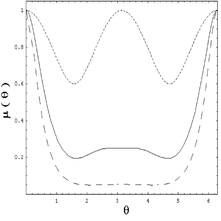
Figure 2: Characteristic exponential factor around a magnetic surface for the main values of the reference surfaces, plain line, and two other situations. No triangularity but Shafranov shift, dashed line, and neither Shafranov and triangularity, point line. The parameters values of the reference curve are: $E=4$, $\tilde{{\Delta}}=0.9$, $A=2.5$, $\tilde{T}=0.3$, $\gamma_{1}=0.3$ and $R_{c}=3\ m$

The dimensionless variables defined previously simplifies the computation, because quantities we need for the calculation are: the ratio between poloidal and toroidal magnetic fields $\gamma_{1}$, the horizontal half-width of the plasma $a$, the aspect ratio $A$, the ratio ${\eta}_{\parallel}/{\eta}_{\perp}$, the Shafranov shift, the ellipticity $K$ and triangularity $\delta$. From $K$ and $\delta$, the values of $E$ and $\tilde{T}$ are determined. The Shafranov shift, the value of $a$ and the calculated value $\tilde{T}$ together allow the calculation of $\tilde{\Delta}$ and $\tilde{\lambda}_{a}$.
In this way the family of magnetic surfaces can be determined. Following the procedures described in previous works the family of orthogonal lines can be also determined, which allows to obtain the curvature function $\kappa_{\sigma}$ and the function $\mu(s)$. All the integrals needed to obtain the normal dimensionless velocity $\tilde{v}$ can also be performed once the value of $\gamma_{1}$ is given. The velocity $\tilde{v}$ can also be obtained if the ratio ${\eta}_{\|}/{\eta}_{\bot}$ is given, and it is a linear function of the dimensionless toroidal electric field $\tilde{E}_{\varphi 1}$. The intersection of that value with the axis of abscissa allows to determine the critical dimensionless electric field $\tilde{E}_{\varphi 1crit}$, for marginal velocity confinement. This field will be later determine for different values of ellipticity $K$, dimensionless Shafranov shift $\Delta_{Shafranov}/a$, and triangularity $\delta$.
Following the above described procedure, the ellipticity $K$ and triangularity $\delta$, in Figure 1, are given as $K=1.76$ and $\delta=0.25$. These correspond to values of $E$ and $\tilde{T}$: $\tilde{E}=4$, $\tilde{T}=0.3$. The real procedure we use was a little different. We first select values of $E$ and $\tilde{T}$, in such way $K$ and $\delta$ become about their values in JET tokamak[8]. This procedure is simpler for us, and it is the same idea.
In Figure 1, several cross sections magnetic lines have been drawn for different values of $\lambda$ in the interval from zero to $\lambda_{a}$, giving in Eq.(24). The characteristic values for that figure are: elipticity $K=1.76$; relative Shafranov shift ${\tilde{\Delta}}_{Shaf}={\Delta}_{Shaf}/a=0.3$; triangularity $\delta=0.25$; horizontal half width $a=1.12\ m$ ( 95 % surface ); aspect ratio $A=2.5$ and minor magnetic axis ratio $R_{c}=3\ m$. From the previous data, the following parameters are determined: elliptic dispersion $E=4$, see Eq.(25)to (27), relative triangularity dispersion $\tilde{T}=T/(E-1)=0.3$; relative Shafranov dispersion ${\tilde{\Delta}}={\tilde{\Delta}}_{Shaf}+\tilde{T}=0.9$; relative $\lambda$-parameter at the 95 % surface $\tilde{\lambda}_{a}=(A+\Delta-T)^{-1}=0.1075$; the outward radius $R_{A_{0}}$, $R1=R(\theta=0)=R_{A_{0}}=R_{c}[1+\tilde{\lambda}_{a}(1+\tilde{T}-\tilde{\Delta})]=3.38\ m$; the inward radius $R2=R(\theta=\pi)=R_{c}[-1+\tilde{\lambda}_{a}(1+\tilde{T}-\tilde{\Delta})]=1.45\ m$; center plasma radius $R_{0}=(R_{1}+R_{2})/2=2.42\ m$ and radius at the maximum z, $((dz/dR)_{R_{m}}=0)$, $R_{m}=2.18\ m$.
In Figure 2, the function $\mu(s)$ is show as a function of $\theta$. This function allows to determine poloidal field around a magnetic surface, once the value $B_{p1}$ at the outward point $A_{0}$ is measured or determined. In order to find $\mu(\theta)$, it is necessary to determine the curvature of the family of orthogonal lines. The procedure has been explained elsewhere[4]. The function $\mu(\theta)$ appears in most of the integrals needed to determine the average normal velocity $<v>\$ first calculated by Pfirsch-Schlüter for cross-sections of circular magnetic surfaces[9]. The function to be used in this work is the central function, plain line. However, two other $\mu$-functions are also shown to illustrate that function. The upper curve correspond to the case where the triangularity and Shafranov shift are zero. The lower curve is just the case of zero triangularity, but the same Shafranov shift than in the main curve ( central one), where the triangularity is $\delta=0.25$, as in Figure 1.
Since the function $\mu(s)$ shown essentially the behavior of $RB_{p}$, the upper curve illustrate that this product is constant at the inward and outward points, when there is not triangularity and Shafranov shift. However, the value of $RB_{p}$, decreases at the uppest and lowest points because of the ellipticity elongation $K=1.76$. The Shafranov shift modifies this pattern in the way that the values at the inward area are almost constant, and very low compared with those at the outward point $A_{0}$. Introducing triangularity as in the case of the central line does not modify the pattern, but the values at the flat part of the curve are not so low.
In Figure 3, the dimensionless average normal velocity is shown as a function of the dimensionless toroidal electric field $\tilde{E}_{\varphi 1}$ at point $A_{0}$, the line here found is the straight line, because of the normalization here used using the value of $(\eta_{\perp}/B_{\varphi})(\partial p/\partial\sigma)_{1}$ at the point $A_{0}$. The intersection of that line with the abscissa define the critical dimensionless toroidal field $\tilde{E}_{\varphi 1}$ for marginal velocity confinement. This critical electric field is show as a function of the elliptic elongation $K$, where all the other variables are kept fixed at the values shown in Figure 1, that is, $\delta=0.25$ and $\tilde{\Delta}=0.9$. To determine the integrals in order to draw Figure 3 and 4, the value of $\gamma_{1}$ is chosen as 0.3, which correspond for instance to toroidal magnetic field $B_{\varphi 1}=5\ Teslas$ and poloidal magnetic field $B_{p1}=1.5\ Teslas$. The ratio of perpendicular to parallel resistivity, ${\eta}_{\parallel}/{\eta}_{\perp}$ has been considered as 1.97 as in page 669 of Ref.(8). As a way of completion $T_{e}$ is taken as $5\ keV$.
The Figure 3 shown that the outward velocity due to diffusion is opposite by the inward effect due to the inductive electric fields $E_{\varphi}$. After a critical value $\tilde{E}_{\varphi}$, the characteristic Ware pinch effect[10] becomes more important, and an average inward velocity $<\tilde{v}>\$ is produced, in such a way that the plasma appears confined as long as instabilities are not considered. The critical dimensionless electric field increase with the elliptic elongation $K$ if all the parameters are kept fixed, however, the variation is not so large, from 0.8 a factor to about 1.1 as it is shown in Figure 4. In this figure has been normalized with a second procedure. First a normalized critical toroidal electric field is selected as reference and denoted by $\tilde{E}_{\varphi 1\ crit.\ ref.}$, which in this case corresponds to that given in Fig. 3, where the characteristic values of the parameters above given. The value of this critical dimensionless toroidal electric field is $29.8106$, and correspond also to the horizontal line through one, which it is also show by a dot line. This kind of normalization is also performed in Figure 5 and 6. The toroidal electric fields with the second normalization explain above are denoted by ${\hat{E}}_{\varphi 1\ crit.}$.
The changes due to Shafranov shift with all the other parameters fixed, are more significative as illustrates the Figure 5, where the critical electric field could be one forth or 3 times the value of that shown in Figure 3. Furthermore the curve in Figure 4 is almost linear, but not that in Figure 5, which seems somewhat as a parabola. Finally, in Figure 6, the change of $\tilde{E}_{\varphi}crit$ with triangularity are shown. There also ${\hat{E}}_{\varphi 1\ crit.}$ changes strongly with $\delta$. More important than this it is that the changes are very significative for low values of $\delta$, and ${\hat{E}}_{\varphi 1\ crit.}$ could be lower by a factor 5, and with values of triangularity no so large, as $\delta=0.25$. Here also the curve is strongly not linear, however the concavity of the curve is opposite to that in Figure 6.

IV Conclusion

In most tokamak operation the inductive magnetic field effect exceeds the plasma diffusion effect and the Ware pinch effect contract the toroidal plasma column. Here the critical point where both effect becomes almost equals is studied. This equilibrium situation is consider as that where the average normal velocity becomes null or void, which will be defined as the marginal velocity confinement. A suitable normalization procedure allows to extend our analysis to a large amount of different situations in tokamak plasma configurations. The critical toroidal electric field changes very little with the ellipticity of the plasma. However, the changes are very strong with the Shafranov shift and triangularity. The curves in those last cases seems parabolas, but with opposite curvature. Very large changes for small values of triangularity have been found, producing changes with a factor 5 for modest triangularity values as $\delta=0.25$.

References

[1] K. H. Burrell, Phys. Plasmas 4, 1499 ( 1997).

[2] V. B. Lebeder and P. H. Diamond, Phys. Plasmas 4, 1087 (1997)

[3] P. H. Diamond, Y. M. Liang B. A. Carreras and P. W. Terry, Phys. Rev. Letters 72, 2565 (1994)

[4] P. Martin and M. G. Haines, Phys. Plasmas 5 410 (1998).

[5] P. Martin, Phys. Plasmas 7, 2915 ( 2000).

[6] P. Martin and J. Puerta, Physica Scripta T-84, 212 (2000).

[7] C. M. Roach, J. W. Connor and S. Janjua, Plasma Phys. Control Fusion 37, 679 (1995)

[8] John Wesson, ” Tokamaks ” ( Clarendon Pres-Oxford, 1997, 2nd Edition ), pp. 555,669.

[9] D. Pfirsch and A. Schlüter, Max-Planck Institute Report MPI/PA/7/62 ( 1962)

[10] A. A. Ware, Phys. Rev. Letters 25 , 15 ( 1970)

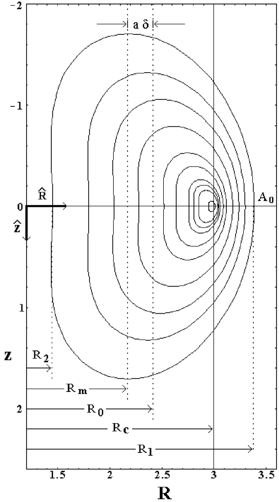
Figure 1: Magnetic flux surfaces showing the characteristic radius, triangularity and main point, with the parameters values given in the text.

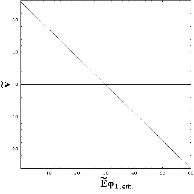
Figure 3: Normalized velocity versus normalized toroidal electric field in the outward point for the parameters values described as reference parameters in the text and for the outward.

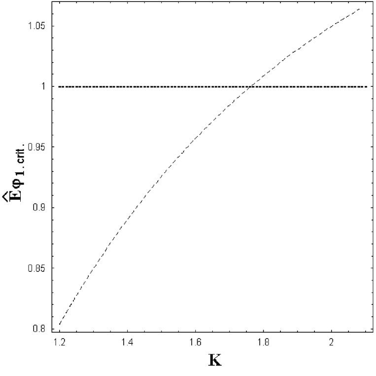
Figure 4: Twofold normalized critical electric field ${\hat{E}}_{\varphi 1\ crit.}$ as a function of elliptic elongation with the triangularity and Shafranov shift equal to those in the reference curves, Fig. 1 and Fig. 3

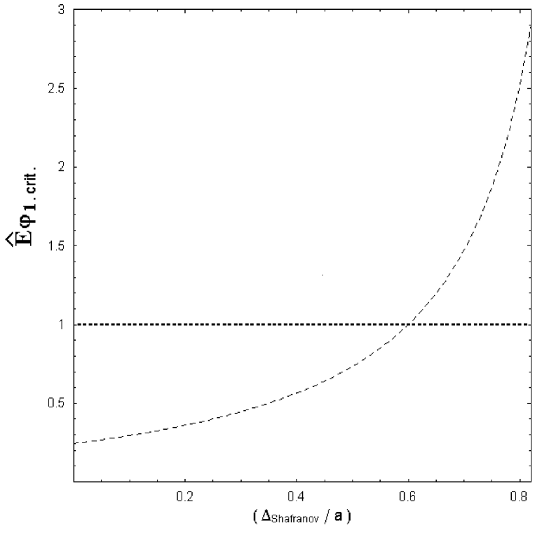
Figure 5: Twofold normalized critical electric field ${\hat{E}}_{\varphi 1\ crit.}$ as a function of dimensionless Shafranov shift with elliptic elongation and Shafranov shift given by the reference curve

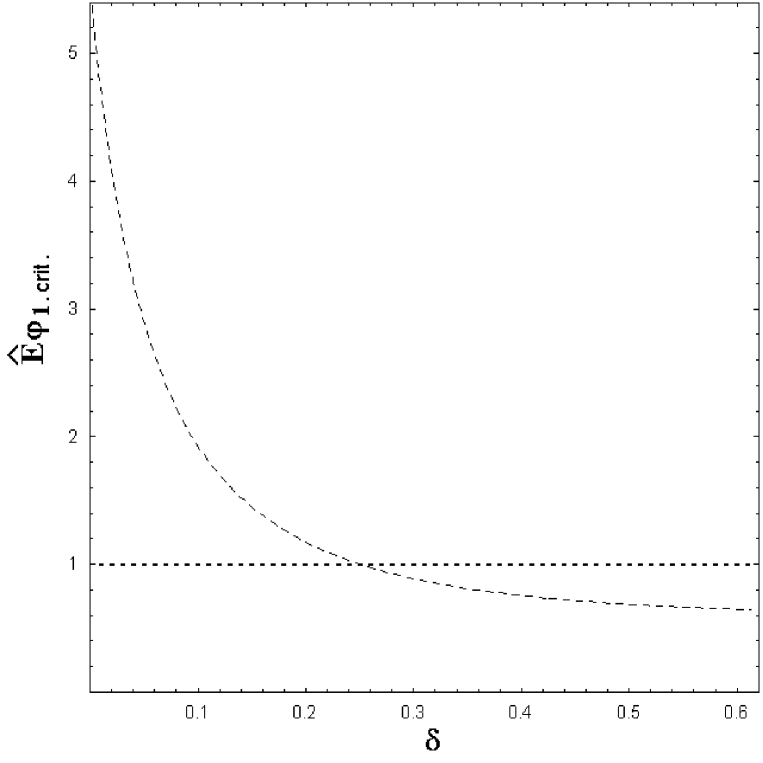
Figure 6: Twofold normalized critical electric field ${\hat{E}}_{\varphi 1\ crit.}$ as a function of triangularity with ellipticity elongation and Shafranov shift given by the reference curve.