Estimation of time delay by coherence analysis

Abstract

Using coherence analysis (which is an extensively used method to study the correlations in frequency domain, between two simultaneously measured signals) we estimate the time delay between two signals. This method is suitable for time delay estimation of narrow band coherence signals for which the conventional methods cannot be reliably applied. We show by analysing coupled Rössler attractors with a known delay, that the method yields satisfactory results. Then, we apply this method to human pathologic tremor. The delay between simultaneously measured traces of Electroencephalogram (EEG) and Electromyogram (EMG) data of subjects with essential hand tremor is calculated. We find that there is a delay of 11-27 milli-seconds ($ms$) between the tremor correlated parts (cortex) of the brain (EEG) and the trembling hand (EMG) which is in agreement with the experimentally observed delay value of 15 $ms$ for the cortico-muscular conduction time. By surrogate analysis we calculate error-bars of the estimated delay.

, , , ,

1 Introduction

The time delay between two dynamical systems can provide information on conduction velocity, and the nature and origin of coupling, between the processes. So it is necessary to use a well validated method for this purpose. Literature on time delay is vast and well documented in [1, 2]. Often, in physiological time series analysis, a single method cannot be made unique to be applicable for a wide class of data stemming from the processes seemingly operated by similar mechanisms. Methods used for time delay estimation are no exception from this fact. Here, we use a spectral based method, maximising coherence, for the time delay estimation [3]. First, we apply this method to uni- and bi-directionally coupled Rössler attractors with a known delay between the systems. In both cases, the results obtained are in good agreement within a narrow range of the delay used in the simulation. Then, we apply this method to simultaneously recorded traces of Electroencephalogram (EEG) and Electromyogram (EMG) of subjects with essential tremor a well known pathological form of hand tremor. We obtain a delay of 11-27 milli seconds ($ms$) between the tremor correlated cortical activity (EEG) and EMG and the results are reasonably within the range of experimentally observed value for cortico-muscular transmission [4]. This result, further confirms the involvement of cortex in the generation of essential tremor [5].

The paper is organised as follows: In section 2, we discuss in detail, the methodology of coherence analysis. Then, we extend the coherence analysis for time delay estimation. Due to a time delay there will be a time misalignment between the two time series thereby causing a reduction in the coherence estimated between them. In order to compensate for the reduction in coherence due to delay, we shift one of the time series keeping the other constant and estimate the coherence as a function of the shift. This method has been successfully applied to estimate the time delay between the acoustic source and the receiving signals [3]. On similar lines, phase synchronisation is used to estimate the time delay between and among the atmospheric variables observed at different meteorological sites [6]. In section 3, we apply this method to afore mentioned theoretical models. After validating the method by the results of standard models, in section 4, we apply this method to estimate the time delay between the simultaneously recorded EEG and EMG data of essential tremor subjects. We discuss the results and conclude in section 5.

2 Methodology

Let $x(t)$ and $y(t)$ be two simultaneously recorded data sets of length $N$. The mean and standard deviation of the two data sets are, respectively, set to zero and one. We divide the data sets into $M$ disjoint segments of length $L$, such that $N=L\cdot M$. We calculate power spectra, $\widehat{S_{xx}}$, $\widehat{S_{yy}}$ and cross spectrum $\widehat{S_{xy}}$, which is the Fourier transform of the cross-correlation function of the signals $x(t)$ and $y(t)$ [1], in each segment. Over cap in all the quantities indicates that it is an estimate of that quantity. Finally, we average the power spectra and the cross-spectrum across all the segments and calculate coherence as follows [7],

$$\widehat{C(\omega)}~{}=~{}\frac{\widehat{|S_{xy}(\omega)}|^{2}}{\widehat{S_{xx}(\omega)}\cdot\widehat{S_{yy}(\omega)}}~{}.$$

The coherence spectrum provides the strength of correlation between the two signals, $x(t)$ and $y(t)$. The confidence limit for coherence at the $100\%~{}\alpha$ is given by $1-(1-\alpha)^{\frac{1}{(M-1)}}$. Thus, the coherence spectrum is always considered with this line. In all of our analysis, $\alpha$ is set to 0.99, and hence the confidence limit is $1-0.01^{\frac{1}{(M-1)}}$. The estimated value of coherence, at a frequency, above this line indicates (a) significant coherence between the two time series at this frequency; (b) the magnitude (deviation of coherence from this line) determines the degree of linear correlation between the two time series at this frequency. The estimated value of coherence at a frequency below this line is considered as the lack of correlation between the two time series at this frequency.

If the sampling frequency of the signals is $sf-$ $Hz$ (i.e. $sf$ number of data points are sampled per second), then the frequency resolution of the quantities in eq. 1, is $\frac{sf}{L}$. Thus, one should optimally choose the value of $L$ depending on the purpose of analysis, to compromise between the sensitivity and reliability. Usage of the fixed segment length $L$ is questioned and a variable segment length is suggested in [8], to make quantitative assessment of the signal. But, for all practical purposes, a fixed segment length is easily implementable and hence, it is used in the forthcoming analysis.

While the coherence spectrum provides the strength of correlation between the two signals $x(t)$ and $y(t)$, time (delay) information between the two signals can be obtained from the phase spectrum, which is the argument of the cross-spectrum [1, 7],

$$\widehat{\Phi(\omega)}~{}=~{}arg\{\widehat{S_{xy}(\omega)\}}.$$

Following [1], eq. 2 can be further simplified to see the explicit appearance of the time delay in it as follows,

$$\widehat{\Phi(\omega)}~{}=~{}\omega\delta,$$

where $\delta$ is the time delay.

The phase estimate $\widehat{\Phi(\omega)}$ and its upper and lower 95% confidence interval are given by [7]

$$\widehat{\Phi(\omega)}~{}\pm 1.96~{}\left[\frac{1}{2M}\left(\frac{1}{\widehat{C(\omega)}}-1\right)\right]^{\frac{1}{2}}.$$

Thus, the confidence interval of the phase estimate is inversely related to coherence. In the rest of the paper we use estimates of the coherence and phase without the over hat for the sake of convenience.

One of the conventional ways to estimate a time delay, in frequency domain, is to fit a straight line to the phase spectrum (eq. 3) in the frequency band of significant coherence, as the phase can be reliably estimated only in the frequency band of significant coherence (see eq. 4). This method of estimating delay is possible when we have a broad band coherence and limits its applicability to the narrow band coherent signals. In some cases, coherence extends to first harmonic and hence the phase values at the harmonics are used to increase the reliability of the delay estimate [9].

Further, if two time series show significant coherence over a wide range of frequency band, but have a minimal phase relation, then the estimation of time delay from the phase estimate is not straight forward. Under such conditions, phase estimate, in addition to the $\omega\delta$ term (see eq. 3), will also contain a frequency dependent factor, namely, the argument of the transfer function, ${\rm{arg}}~{}A(\omega)$. In such cases, ${\rm{arg}}~{}A(\omega)$ is estimated by Hilbert transform, and then delay is estimated from the phase estimate after subtracting the estimated transfer function from the phase estimate [2]. From the above discussion it is clear that phase estimates cannot be used to estimate the delay from narrow band coherent signals which are often observed in human physiological data [5, 10]. For this purpose, we use the method of maximising coherence.

As discussed in the last part of the introduction, a delay $\delta$ between two time series, will cause a reduction in the estimated coherence between them. In order to compensate for the reduction in coherence due to delay and thereby to estimate the delay, we realign the time series by artificially shifting them. For this, we shift one of the time series by a lag $(\tau)$ keeping the other constant and consider coherence at the selected frequency band $\omega_{0}$ as a function of $\tau$, $C(\tau)_{\omega_{0}}$ and repeat the same for the other time series. If there is a delay between the two time series, coherence in the selected frequency band $C(\tau)_{\omega_{0}}$ will increase from its value at $\tau=0$ and reach a maximum at the $\tau$ corresponding to $\delta$. After shifting one of the time series by a lag $\tau$, the length of the shifted time series will be less than the un-shifted time series by $N-\tau$ ($\tau$ in sample units) data points. We discard the extra data points in the un-shifted time series to have the same length for both time series. Further, coherence is a relative measure and changes with the length of the data. It is reflected in the 99% confidence level (see above). For each shift, we discard the points corresponding to the maximum lag from the entire length of the time series, and consider only the length of the data which is integer multiple of $L$. By doing so, coherence $C(\tau)_{\omega_{0}}$ calculated for all the lags will have the same confidence level, thereby confirming that the maximum value of coherence is reached only because of the delay and not due to the spurious effects caused in estimating coherence for different lengths of data. As we have confidence level as a check for the reliability of $\delta$, we don’t need any additional tests like, surrogate tests [11] to assess the reliability of the results. However, in order to get the variability in the estimated delay, we use surrogate analysis.

Surrogate analysis is introduced in the context of nonlinear time series analysis to check whether or not the time series under consideration has got a nonlinear structure [11, 12]. Making the (null) hypothesis that the time series has come from a linear process, several linear realizations of the time series namely, surrogates, are synthesised. Then, the original time series and the surrogates are quantified by a suitable discriminating statistic. Any deviation in the discriminating statistic calculated for the original time series and surrogates indicates the presence of nonlinear structure in the original time series and thereby rejecting the null hypothesis [12]. There are different ways of preparing the surrogates [11, 13]. The misconception of surrogate analysis is discussed in [14]. As mentioned above, the objective of the methods to generate surrogates [11, 13] is to synthesise a new data set by destroying the nonlinear structure present in the original data set. But our aim is not to show the presence of nonlinear structure in our data. For the purpose of calculating the error-bars of delay, surrogates are generated by exploiting one of the basic assumptions of spectral analysis that distinct parts of the time series are independent [7]. Instead of shuffling the time series as a whole (which is done in one of the methods to synthesise surrogates, amplitude adjusted surrogates) we shuffle the disjoint data segments from which the original spectrum is estimated (see above). We shuffle only the un-shifted time series (see above) from which the information is assumed to flow to the other time series (which is time shifted in advance in maximising coherence analysis) with a delay. By doing so, the spectra of both the time series, $\widehat{S_{xx}(\omega)}$ and $\widehat{S_{yy}(\omega)}$ in eq. 1 will remain the same but the cross spectrum $\widehat{S_{xy}(\omega)}$ in eq. 1 will be different. This type of surrogate is similar to the one proposed in [13] where the whole time series is shuffled but by preserving two point correlation (i.e. power spectrum) of the original time series. For all the analyses reported in this paper we synthesise 19 different realizations of surrogates. We make a null hypothesis that $C(\tau)_{\omega_{0}}$ obtained is due to spurious correlations between the two time series. For each realization of surrogate we calculate time delayed coherence $C(\tau)_{\omega_{0}}^{surr}$. We calculate the significance of difference $S(\tau)$ between the $C(\tau)_{\omega_{0}}^{surr}$ calculated for surrogates and $C(\tau)_{\omega_{0}}$ where $S(\tau)=\frac{\left|C(\tau)_{\omega_{0}}-<C(\tau)_{\omega_{0}}^{surr}>\right|}{\sigma[C(\tau)_{\omega_{0}}^{surr}]}$, where $<.>$ indicates the average over different realizations of surrogates and $\sigma[.]$ indicates the standard deviation between different realizations of surrogates. Any value of $S(\tau)>2$ indicates that the $C(\tau)_{\omega_{0}}$ obtained is not due to spurious correlations [12] and hence the null hypothesis is rejected. If the null hypothesis is rejected we consider $C(\tau)_{\omega_{0}}$ for further analysis otherwise we discard it as spurious correlation. For the $C(\tau)_{\omega_{0}}$ qualified in the surrogate analysis (for which null hypothesis is rejected) we calculate the error in the delay in the following way: we subtract $C(\tau)_{\omega_{0}}^{surr}$ calculated for each realization from $C(\tau)_{\omega_{0}}$ and calculate delay for each subtracted function (i.e.) $C(\tau)_{\omega_{0}}-C(\tau)_{\omega_{0}}^{surr}$. We report here the delay of the system as the mean value of the delays (calculated for the 19 surrogate subtracted realizations) and their standard deviation as error-bar. As the increase in the $C(\tau)_{\omega_{0}}$ when compensated for the delay is very small, for the sake of clarity we plot $C^{\prime}(\tau)_{\omega_{0}}=\left[C(\tau)_{\omega_{0}}-<C(\tau)_{\omega_{0}}^{surr}>\right]-\left[C(\omega_{0})-<C(\omega_{0})^{surr}>\right]$. Note that $C(\omega_{0})$ is the value of $C(\tau)_{\omega_{0}}$ at $\tau=0$ and $<C(\omega_{0})^{surr}>$ is the average of $C(\tau)_{\omega_{0}}^{surr}$ for different realizations of the surrogates at $\tau=0$. By this definition $C^{\prime}(\tau)_{\omega_{0}}$ will pass through a zero value at $\tau=0$ and show a maximum value (above zero) at $\tau=\delta$ (for $\delta\neq 0$) between the processes. Though we calculate $S(\tau)$ for different $\tau$ values at which $C(\tau)_{\omega_{0}}$ is evaluated, we report here $S(\tau=\delta)$ as it is the most relevant one in determining the significance of the $C^{\prime}(\tau=\delta)_{\omega_{0}}$ (and hence $C(\tau=\delta)_{\omega_{0}}$). Based on the above arguments the delay between the two time series is given by:

$$\delta={\max_{\tau}}~{}C^{\prime}(\tau)_{\omega_{0}}.$$

3 Application to coupled Rössler attractors

In this section, we apply the method of maximising coherence, to coupled Rössler systems. The dynamics of the $i$-th attractor is given as follows:

$$\dot{x}_{i}(t) = -[y_{i}(t)-z_{i}(t)]~{}+~{}\epsilon_{j,i}~{}x_{j}(t-\delta)$$

$$\dot{y}_{i}(t) = x_{i}(t)~{}+~{}a~{}y_{i}(t)$$

$$~{}\dot{z}_{i}(t) = b~{}+~{}z_{i}(t)~{}[x_{i}(t)~{}+~{}c],$$

where $a~{}=~{}0.38,~{}b~{}=~{}0.3,~{}c~{}=~{}4.5$, are the parameters. Coupling is established through the $x$ component between the attractors. $\epsilon_{j,i}$, is the coupling constant and $x_{j}$ is the $x-$ component of the $j-$th attractor. In our study, we consider the dynamics of two coupled Rössler attractors, and hence $i~{}=~{}1$ and $j~{}=~{}2$ and $\delta$ is the delay. Further, we don’t consider the self coupling of the oscillators.

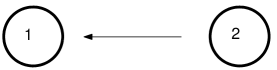
Figure 1: Coupling scheme of the attractors 1 and 2. $\epsilon_{2,1}=0.16$ and $\epsilon_{1,2}=0$. $\delta$ is set to 2 sec.

First, we consider the coupling scheme as shown in Fig. 1, where two Rössler attractors are coupled and the information flow is from attractor 2 to attractor 1 ($\epsilon_{2,1}=0.16$ and $\epsilon_{1,2}=0$) as governed by the above set of equations. $\delta$ is set to 2 sec. The above equations are simulated by Euler scheme with a step size of 0.01 sec and for the subsequent analysis the data are down sampled to 0.1 sec. As the coupling is established through the $x-$ component between the attractors, we use the $x-$ time series to perform the delay estimation. We have used 30000 data points for further analysis.

Power spectra of the two attractors are shown in Fig 2a. Solid line represents the power spectrum of attractor 1 and solid line with dots represents the power spectrum of attractor 2. For the sake of clarity the spectrum of attractor 1 is shifted vertically upwards by a factor of 5 from its original position. We have used a segment length of $L=1000$ and hence the frequency resolution (of the quantities in eq. 1) is 0.01 $Hz$. Spectra show dominant activities in the frequency range of 0.1 to 0.2 $Hz$, which can be related to the mean orbital period of $\sim 5$ sec of the attractor [15, 16]. Since the dynamics of the attractor 1 is perturbed by coupling (see Fig. 1), its spectrum looks slightly different from that of the attractor 2. The coherence spectrum of the coupled attractors is shown in Fig. 2b. Horizontal line around the coherence of 0.15 indicates the confidence level of $\alpha=0.99$.

In the frequency band between 0.1-0.2 $Hz$ (see Fig. 2a), where the individual attractors show dominant activities, the coupled systems show significant coherence. Estimated phase (eq. 2) between the coupled attractors is shown in Fig. 2c. Error-bars represent the 95% confidence interval of the phase estimate given by eq. 4. Thus the phase can be reliably estimated in the frequency band (0.1-0.2 $Hz$), where the coupled attractors show a significant coherence (see Fig. 2b). The result of maximising coherence is shown in Fig. 2d where $C^{\prime}(\tau)_{\omega_{0}}$ is plotted as a function of lag $\tau$. We have chosen $\omega_{0}=0.13Hz$ (and is shown in Fig. 2b) from the basic frequency of the oscillators. Solid line at $C^{\prime}(\tau)_{\omega_{0}}=0$ indicates $C(\omega_{0})-<C(\omega_{0})^{surr}>$(see the last part of the methodology for details). Negative shift indicates that the time series of attractor 1 is in advance and positive shift indicates that the time series of attractor 2 is in advance. Since there is a delay of 2 sec, the coherence calculated at $\tau=0$ is zero (see above). In order to compensate for the reduction in the coherence and thereby to estimate the time delay, time series of the attractors are shifted by a time lag $\tau$. As the delayed information flows from attractor 2 to attractor 1, coherence $C^{\prime}(\tau)_{\omega_{0}}$ increases from zero (see above) when the time series of attractor 1 is shifted back in time and reaches a maximum at the $\tau=-2.1$ which is the time delay between the two time series ($\delta$ used in the simulation is 2 sec). The significance of deviation from the surrogate data $S(-2.1)$ is 2.24 and indicates that $C^{\prime}(\tau=-2.1)$ is not due to spurious correlations. The error-bar for the delay (as explained in the methodology section) is calculated as 0.4 sec. Thus, the time delay $\delta$ is $-2.1\pm 0.4$ sec and is well captured by the maximising coherence analysis (expected delay value is 2 sec for the flow from attractor 2 to attractor 1).

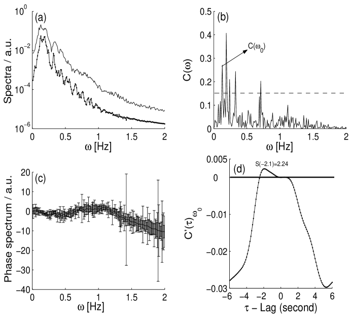
Figure 2: (a). Solid line represents power spectrum of attractor 1 and solid line with dots represents power spectrum of attractor 2. For the sake of clarity the power spectrum of attractor 1 is shifted vertically upwards by a factor of 5 from its original position. (b). Estimated coherence spectrum of the coupled Rössler attractors with $\delta=2$ sec. Horizonal line at the coherence of 0.15 indicates the confidence level ($\alpha=0.99$). There is a significant coherence in the frequency range of 0.1-0.2 $Hz$ between the two attractors. The value of $\omega_{0}$ used for maximising coherence analysis is indicated along with its coherence value $C(\omega_{0})$. (c). Phase estimate $\Phi(\omega)$ of the coupled attractors. Error-bars represent 95% confidence interval defined by eq. 4. Errors are relatively small in the region of significant coherence which is in accordance to eq. 4. (d). Coherence $C^{\prime}(\tau)_{\omega_{0}}$, as the function of lag $\tau$. Horizontal line at $C^{\prime}(\tau)_{\omega_{0}}=0$ indicates $C(\omega_{0})-<C(\omega_{0})^{surr}>$. $<.>$ represents the average over different surrogates. $C^{\prime}(\tau)_{\omega_{0}}$ has reached the maximum value at the $\tau$ (delay) value of -2.1 sec (from attractor 2 to 1), and the expected value of $\delta$ is 2 sec for the flow from attractor 2 to attractor 1. The significance of deviation from the surrogate $S(-2.1)$ is 2.24 and indicates that $C^{\prime}(\tau)_{\omega_{0}}$ is not due to spurious correlations.

Next, we consider the coupling scheme as shown in Fig. 3, where two Rössler attractors are coupled as considered above, but with a bi-directional flow, $\epsilon_{2,1}=0.15$ and $\epsilon_{1,2}=0.1$. $\delta$ used in the coupling is same as in Fig. 1, which is 2 sec.

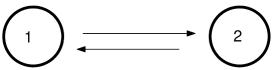
Figure 3: Coupling scheme of the attractors 1 and 2. $\epsilon_{2,1}=0.15$ and $\epsilon_{1,2}=0.1$. $\delta$ is set to 2 sec.

Power spectra of the attractors look almost the same as the two attractors perturb each other almost to the same extent (see Fig. 4a). As obtained for uni-directional coupling, in this case also, significant coherence is between 0.1-0.2 $Hz$ (Fig. 4b). As the number of data points used is the same (30000) as in the uni-directional coupling, the confidence level $\alpha=0.99$ is also around the coherence of 0.15 (see the horizontal line in Fig. 4 b which is same as in Fig. 2b). Phase estimate of the bi-directionally coupled systems is shown in Fig. 4c with the 95 % confidence interval as the error-bars. Error-bars are relatively narrow (see eq. 4) in the frequency band of 0.1-0.2 $Hz$ where significant coherence is observed (as seen in Fig. 2c). Result of the maximising coherence for bi-directionally coupled systems is shown in Fig. 4d. The horizontal line at $C^{\prime}(\tau)_{\omega_{0}}=0$ has the meaning as in Fig. 2d. In this case 0.15 $Hz$ is used as $\omega_{0}$ (and is shown in Fig. 4b) which is the basic frequency of the attractors. $C^{\prime}(\tau)_{\omega_{0}}$ shows two maxima, one at $\tau=-2.5$ sec which corresponds to the flow from attractor 2 to 1 and another at $\tau=1.7$ sec which corresponds to the flow from attractor 1 to 2, while the $\delta$ used in the coupling is 2 sec in both directions (see Fig. 4d). Also, in this case, the significance of deviation from surrogate calculated by $S(\tau)$ at $\tau$ values -2.5 sec and 1.7 sec are well above 2 (see Fig. 4d) indicating that the $C^{\prime}(\tau)_{\omega_{0}}$ obtained at these two $\tau$ values are not due to spurious correlations. Thus, the time delays of the system are $-2.5\pm 0.5$ sec (for the flow from attractor 2 to attractor 1) and $1.7\pm 0.4$ sec (for the flow from attractor 1 to attractor 2) and are well within the expected value of 2 sec in either direction (see Fig. 3). The error-bars are obtained by surrogate analysis.

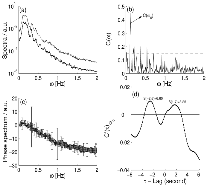
Figure 4: (a-c). Explanations are as in Fig. 2 but for bi-directionally coupled Rössler attractors, $\epsilon_{2,1}=0.15$ and $\epsilon_{1,2}=0.1$. (d). Result of maximising coherence $C^{\prime}(\tau)_{\omega_{0}}$. $C^{\prime}(\tau)_{\omega_{0}}$ has reached maximum value at two places, one at -2.5 sec (from attractor 2 to 1) and another at 1.7 sec (from attractor 1 to 2), where $\delta$ is set to 2 sec in both directions. The significance of deviation from surrogate at $S(-2.5)$ is 6.60 and at $S(1.7)$ is 3.25 and indicates that $C^{\prime}(\tau)$ at $\tau$ values -2.5 sec and 1.7 sec are not due to spurious correlations. The horizontal line at $C^{\prime}(\tau)_{\omega_{0}}=0$ has the same meaning as in Fig. 2d.

Results of the theoretically coupled systems are summarised in Fig. 5. For the unidirectional flow, shown in Fig. 1, which is referred to as scenario 1 in Fig. 5, the value of the delay obtained by maximising coherence, shown by ’$\ast$’ with the error-bars (calculated by surrogate analysis) shown as vertical line, is close to the expected value of -2 sec (shown as dot in Fig. 5). Similarly for the bi-directional flow (see Fig. 3) which is referred to as scenario 2 in Fig. 5, the values of the delay obtained by maximising coherence with their error-bars (vertical lines) are close to the expected delay of 2 sec in either direction (see Fig. 3). Compared to the unidirectional flow, the results of the bi-directionally coupled oscillators show slightly more deviations from the expected value of 2 sec but when we include the error-bar, they are close to the expected value. So when dealing with the biological systems we should consider the delay always with the error-bar before we draw any conclusion from it. For the uni-directionally coupled oscillators there is no significant change in the result when $\omega_{0}$ is chosen as 0.19 $Hz$ where there is a significant coherence between the two oscillators. Further for the above studied systems similar results can be obtained by cross-correlation analysis and by the time delayed phase synchronisation analysis as well [6].

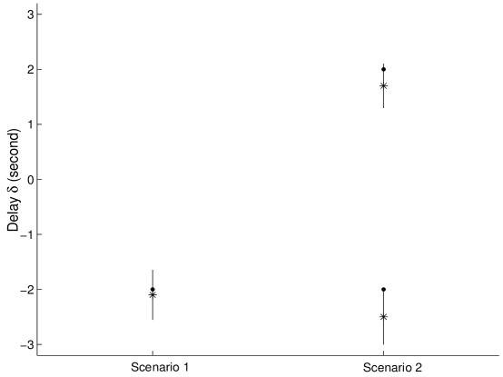
Figure 5: Results of delay estimation by maximising coherence for theoretically coupled systems. Negative delay indicates the flow from attractor 2 to attractor 1 and the positive delay indicates the flow from attractor 1 to attractor 2. Scenario 1 represents uni-directionally coupled oscillators (flow from attractor 2 to attractor 1). Scenario 2 represents bi-directionally coupled oscillators. Expected delay values are shown by dots. Delay values obtained by maximising coherence are shown by ’$\ast$’. Vertical lines are the error-bars of delay (see text for details).

4 Application to EEG and EMG data

Tremor is an involuntary, periodic movement of the parts of the body [17]. It can be classified as normal and pathological tremor depending on amplitude and the conditions under which tremor is activated [17]. Essential tremor is a common movement disorder characterised mostly by postural tremor of the arms. Other neurological abnormalities are typically absent in essential tremor [18]. It has been shown by experimental studies in animals [19, 20] and by Positron emission tomography or functional magnetic resonance imaging studies [21, 22, 23] on human beings, that different parts of the brain are involved in essential tremor. The correlation between the thalamic activity and forearm electromyogram provides a direct evidence for the involvement of the thalamus in the tremor oscillations [24]. Further, control of essential tremor by stereo-tactic lesions and high frequency stimulation of the ventrolateral thalamus adds support for the involvement of thalamus in the mechanism of essential tremor [25, 26]. As the cerebellum has its main outputs to thalamus which in turn has strong projections to cortex, it is hypothesised that essential tremor arise from an oscillating cerebello-thalamo-cortical loop the output station of which is the motor cortex [5].

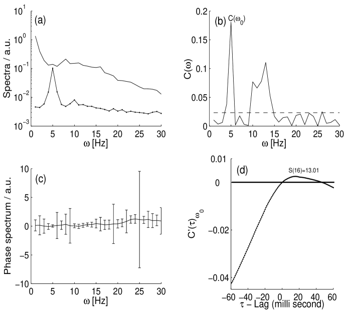
Figure 6: Results of spectral analysis and delay estimation for subject 1. (a). Solid line represents power spectrum of C4 of EEG (the central electrode overlaying the primary motor cortex, PMC) and solid line with dots represents the power spectrum of extensor muscle with a frequency resolution of 1 $Hz$. For the sake of clarity, the power spectrum of EEG is shifted vertically upwards from its original position by a factor of 10. (b). Coherence spectrum of C4 and extensor muscle. The horizontal line at the coherence of 0.024 indicates the confidence level of $\alpha=0.99$. There is a significant coherence at the (tremor) frequency of 5 $Hz$ and at 10-15 $Hz$ as well. The value of $\omega_{0}$ used for the maximising coherence is shown along with its coherence value $C(\omega_{0})$. (c). Phase estimate of the C4 and extensor muscle with 95% confidence interval as the error-bars. Error-bars are narrow at the significantly coherent frequency bands of 5 $Hz$ and 10-15 $Hz$ as well. (d). Coherence as a function of $\tau$, $C^{\prime}(\tau)_{\omega_{0}}$. It has reached maximum at $\tau=16$ $ms$. The horizontal line at $C^{\prime}(\tau)_{\omega_{0}}=0$ has the same meaning as in Fig. 2d. The significance of deviation from the surrogate is given as $S(16)=13.01$.

Cortico-muscular coherence for essential tremor has been studied earlier [27] but has not been ascertained at the tremor frequency in [27]. We show below that there is a significant cortico-muscular coherence when the signal to noise ratio of the tremor increases beyond a certain threshold value as seen in [5, 28]. Since the paper is aimed at time delay estimation, the detailed results and discussion of the spectral analysis of the tremor study will be reported elsewhere [10].

For this purpose we consider five patients (with mean age 66 years and standard deviation 5.1 years), which showed postural essential tremor of the arms. In a dimly lighted room, patients are asked to sit on a comfortable chair in a slightly supine position with both hands held against gravity while the forearms are supported. EEG is recorded with a 64-channel EEG system (Neuroscan) with standard electrode positions [29]. Surface EMG is recorded from EMG electrodes attached to wrist flexors and extensors of both arms. For all the subjects EEG and EMG are sampled at a rate of 1000 $Hz$. EEG and EMG are bandpass filtered online, respectively, between 0.01-200 $Hz$ and 30-200 $Hz$. Data are stored in a computer and are analysed offline. In all the cases EMG is recorded on both hands. Each recording lasted for 1-4 minutes. Artifacts like base line shift, eye blinks etc. are discarded by visual inspection.

Before further analysis, EMG signals are full wave rectified (magnitude of the deviations from mean) and EEG is made reference free by constructing the second (spatial) derivative, (Laplacian) [30, 31]. We discuss in detail for one of the subjects, subject 1, which we feel typical and for the remaining subjects we summarise the results in a table.

For subject 1, the power spectra of EEG (solid line) and EMG (solid line with dots), see Fig. 6a, are calculated with $L=1000$ and hence the frequency resolution is 1 $Hz$ (since $sf=1000$ $Hz$). In Fig. 6a, we show the power spectra of one of the EEG channels (C4) in the contralateral (right) side to tremor (left) hand and the rectified EMG (extensor muscle) of the same hand. Power spectrum of EEG (shown as solid line in Fig. 6a) is shifted vertically upwards by a factor of 10 from its initial position for the sake of clarity. Power spectrum of EEG shows dominant activity in a broad band between 8-20 $Hz$ containing the bands of 10-13 $Hz$ and 15-20 $Hz$, which correspond, respectively, to the alpha and beta activity of the brain [32]. Muscle spectrum (solid line with dots in Fig. 6a) shows tremor activity around 5 $Hz$. Correlation between the muscle and C4 (the central electrode overlaying the primary motor cortex, PMC) of EEG cannot be guessed from the EEG spectrum as there is no significant activity around 5 $Hz$ (tremor frequency). Correlation becomes clear when we consider coherence. Figure 6b shows coherence between C4 and extensor muscle. The horizontal line around the coherence of 0.024 indicates the confidence level of $\alpha=0.99$. There is a significant coherence (and hence correlation) between C4 and the tremor activity reflected by the muscle [5, 28, 33, 34, 35, 36] and also in the frequency band of 10-15 $Hz$. Phase estimate of this system is given in Fig. 6c with $95\%$ confidence interval as error-bars. It is clear from Fig. 6c that phase can be reliably estimated at the (tremor and the significant coherence) frequency of 5 $Hz$ (confidence interval is narrow) and also in the frequency band of 10-15 $Hz$. In an earlier study Hellwig et al. [28] investigated time delays based on the value of the phase estimate $\widehat{\Phi(\omega)}$ at the tremor frequency. But the results obtained [28] are not in the interpretable level. The reason postulated in [28] that the delay might be modulated by frequency dependent mechanism is hardly conceivable in a narrow (single) frequency band at which phase estimate is significant. The reason may be due to the weak assumption of the model $\widehat{\Phi(\omega)}=\omega\delta+\theta$, where $\theta$ is the indispensable constant [33, 34], phase shift between the two processes which is ignored in [28]. However, we show below that the delay estimated by maximising coherence is reasonably in good agreement with the experimentally observed conduction velocity and is in physiologically interpretable range.

Application of the maximising coherence method to real life data like EEG is not straight forward. Since the maximising coherence method is aimed at to capture the time delay (by making up for the reduction in the coherence) by artificially shifting (local dynamics) the time series, it is very sensitive to non-stationarities in the time series. However, in order to make coherence analysis robust against non-stationarities within the time series, we use the following way to discard the non-stationary parts of the data: We calculate autocorrelation function [37], in each of the segments (of length 1000 samples). Then the de-correlation time, time at which autocorrelation function falls to $exp(-1)$ (as the first value of autocorrelation function is 1 by definition) [37] is calculated for all the segments. Non-stationarities due to base line shift, eye blinks will introduce artificial trends (lifting up of the mean value of the signal) [38] in the signal, which will have higher de-correlation time than the stationary parts of the signal. In order to discard the non-stationary parts, about 50 % of the median of the de-correlation time calculated in all the segments is taken as threshold and parts of the EEG and EMG data with de-correlation time greater than the above defined threshold are discarded in the delay estimation. After discarding the non-stationary parts of the data, the segments left out on either side of the removed parts are stitched as if they are recorded continously. Of course, care should be taken in applying the above method. The above method will capture only the non-stationary parts if it is applied to the data of low signal to noise ratio which can be avoided by visual inspection of the data.

Result of the delay estimation between C4 and muscle, is shown in Fig. 6d. The horizontal line at $C^{\prime}(\tau)_{\omega_{0}}=0$ in Fig. 6d has the same meaning as in Fig. 2d. Here, we have used $\omega_{0}=5$ $Hz$ (see Fig. 6b), where significant coherence is observed. Negative shift indicates that the time series of EEG is in advance. In Fig. 6d, $C^{\prime}(\tau)_{\omega_{0}}$ reaches a maximum value at $\tau=16$ $ms$, indicating the cortex (time series of EMG is in advance for positive values of $\tau$) is driving the tremor. The significance of deviation from the surrogate is given by $S(16)=13.01$ and indicates that $C^{\prime}(\tau)_{\omega_{0}}$ obtained is not due to spurious correlations. The error-bar obtained by surrogate analysis is 7 $ms$ and hence the delay obtained for C4 is 16$\pm$7 $ms$ which is in good agreement with the experimentally observed value of around 15 $ms$ [4]. Comparison of Fig. 6d with Fig. 2d, shows that the information flow is in one direction (i.e.) from cortex to muscle. But in other subjects, in (an electrode from) this region, we have also observed a bi-directional flow, a situation similar to Fig. 4d.

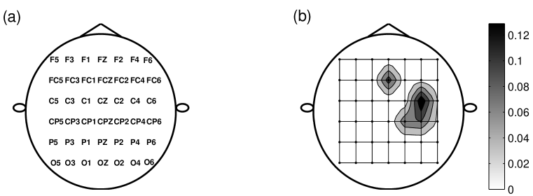
Figure 7: (a). A part of the 64-channel arrangement on the surface of the scalp used to record EEG. Electrodes on the left hand side are odd numbered and those on the right hand side are even numbered. (b). Isocoherence map of the subject 1, constructed by considering the coherence at the tremor frequency (5 $Hz$ in this case). Magnitude of the coherence is indicated by the gray scale-bar juxtaposed to the isocoherence map. Parts of the scalp which showed significant coherence are coloured black and the confidence level of $\alpha=0.99$ is marked with white colour (which is set to zero, see text for details). (Electrodes O5-O6 are just displayed and are not used for coherence analysis).

Of the 64-channels of EEG recorded, coherence and delay estimation are explained in detail for C4, as it is overlaying the primary sensorimotor cortex which is involved in motor control of the contralateral hand affected by essential tremor. For the rest of the electrodes (see Fig. 7a) we give the results of the coherence analysis as isocoherence (region of scalp with same coherence) map. Electrodes on the boundary of the scalp are not considered for the analysis as they had low signal to noise ratio. Further, we have not used the electrodes O5 - O6 for the study. To construct isocoherence map, we have considered the coherence $C(\omega)$ at the (tremor) frequency of 5 $Hz$ for all the thirty five channels (see above) shown in Fig. 7a, from F5 (top left of scalp, Fig. 7a), to P6 (bottom right of scalp, Fig. 7a). We have subtracted the confidence level ($\alpha=0.99$) from the coherence so that the confidence level for coherence is zero. In Fig. 7b, surface of the scalp exhibiting significant coherence is marked with black colour and the coherence of the parts which do not cross the confidence level of $\alpha=0.99$ (which are set to zero after the above normalisation) are marked with white colour. In Fig. 7b, C4 shows maximum coherence, (see the gray scale-bar juxtaposed to Fig. 7b). Thus, there is a hot spot (region of significant coherence) in the PMC region. Similar results have been obtained in the spectral study of essential tremor [5, 28].

There is another hot spot for subject 1 in the frontal region of the scalp (FCZ). The detailed discussion of this will be dealt with in [10].

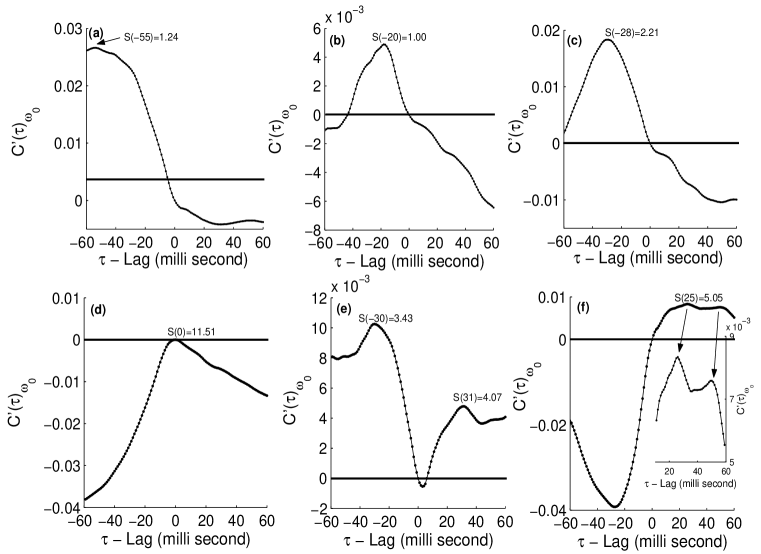
Figure 8: Results of delay estimation by maximising coherence for (a). C2 (b). C6 (c). CP2 (d). CP4 (e). CP6 of the central hot spot and (f). FCZ of the frontal hot spot. The horizontal line at $C^{\prime}(\tau)_{\omega_{0}}=0$ in Fig. 8 (a-f) has the same meaning as in Fig. 2d. The significance of deviation from the surrogate $S(\tau)$ at $\tau=\delta$ is given in all the plots. Estimated values of delay by maximising coherence are (c) -28 $ms$ (d) -2 $\sim$ 0 $ms$ (e) -30 $ms$ and 31 $ms$ (f) 25 $ms$. As the maximum of $C^{\prime}(\tau)_{\omega_{0}}=25~{}ms$ in Fig. 8f is not clearly discernable (see text for details) it is magnified in the inset shown in Fig. 8f. Negative shift indicates that the time series of EEG is in advance and positive shift indicates that the time series of EMG is in advance. A negative delay indicates the flow from muscle to EEG and a positive delay indicates the flow from EEG to muscle. C2 and C6 do not qualify in the surrogate analysis as their $S(\tau=\delta)$ values lie below 2 indicating that the values of $C^{\prime}(\tau)_{\omega_{0}}$ (see Fig. 8a and 8b) obtained for these two electrodes are due to spurious correlations and therefore are not considered for further analysis.

Spectral and delay estimations for C4 and extensor muscle have been analysed in detail showing a uni-directional flow from PMC to muscle, with a delay of 16 $ms$. For the rest of the electrodes (C2, C6, CP2, CP4, CP6) of the central hot spot and FCZ of the frontal hot spot, the results of delay estimation are given in Fig. 8. The significance of deviation from surrogate $S(\tau)$ at $\tau=\delta$ is given in all the plots, see Fig. 8(a-f). For C2 (Fig. 8a) and C6 (Fig. 8b) the value of $S(\tau=\delta)$ is below two indicating that the values of $C^{\prime}(\tau)_{\omega_{0}}$ obtained for these two electrodes are due to spurious correlations. Therefore we do not consider them for further analysis. For CP2, CP4, CP6 and FCZ, $S(\tau=\delta)$ values obtained are above 2 (see Fig. 8(c-f)) indicating that $C^{\prime}(\tau)_{\omega_{0}}$ values obtained for these electrodes are not due to spurious correlations. Delay values exhibited by $C(\tau)_{\omega_{0}}$ shown in Fig. 8(c-f) are CP2 -28 $\pm$ 3.3 $ms$ (see Fig. 8c), CP4, -2 $\sim$ 0 $ms$ (see Fig. 8d), CP6 -30 $\pm$ 7.4 and 31 $\pm$ 13.5 $ms$ (see Fig. 8e) and FCZ 25 $\pm$ 10.4 $ms$ (see Fig. 8f). The maximum in $C^{\prime}(25)_{\omega_{0}}$ for FCZ shown in Fig. 8f is not clearly discernable and hence this region is magnified in the inset shown in Fig. 8f where the maximum at $\tau=25~{}ms$ can be seen without any ambiguity. The large fluctuations in $C^{\prime}(\tau)_{\omega_{0}}$ for FCZ (Fig. 8f) and C4 (Fig. 6d) indicate larger uncertainty in the delay estimated by this method and is one of the shortcomings of this method. However, this uncertainty, to some extent is revealed by the error-bars (see above) obtained by the surrogate analysis. A positive value of $\tau$ indicates that the time series of muscle is in advance and a negative value of $\tau$ indicates that the time series of EEG is in advance. Error-bars are obtained by surrogate analysis as discussed in the methodology section. A zero delay for CP4 (see Fig. 8d) may be due to the nullification of two strong counter acting forces (drive from PMC to muscle and opposing drive from muscle to PMC, a situation similar to phase locking in coupled oscillators). The positive values of estimated delays including the error-bars are well in agreement with the experimentally observed value of 15 $ms$ for forearm muscles [4]. For the negative delay (flow from muscle to EEG), it is at least partly in keeping with normal median Somatosensory Evoked Potential (SEP) latencies of around 20 $ms$.

Further, in order to make the delay statistically significant we report the delay of the hot spot as a whole as the delay of the system, by weighting the delay obtained for each electrode (when it is qualified in surrogate analysis) by a fraction of the coherence $C(\omega_{0})$ value that each electrode contributes to the hot spot. By doing so, electrodes showing higher tremor related correlations will contribute more to the delay of the system. For subject 1, there is a hot spot (central hot spot) in the PMC region of scalp and another in the frontal region of the scalp (i.e.) FCZ (see Fig. 7b). Of the electrodes contributing to the central hot spot, we do not consider C2 and C6 (as they do not qualify in the surrogate analysis) for further analysis. We weight the delay obtained for rest of the electrodes contributing to the central hot spot by $NC^{(l)}(\omega_{0})=\frac{C^{(l)}(\omega_{0})}{\sum_{j=1}^{K}C^{(j)}(\omega_{0})}$, where $K$ is the number of electrodes contributing to hot spot after qualifying the surrogate analysis, and $[100\cdot NC^{(l)}(\omega_{0})]$ % is the contribution of the $l-$th electrode to the hot spot (it is easy to check that $\sum_{j=1}^{K}NC^{(j)}(\omega_{0})=1$). Similarly $NC^{(l)}(\omega_{0})$ is calculated for each hot spot. Further, in the calculation of $NC^{(l)}(\omega_{0})$ for positive delay, only those electrodes which display positive delay are considered and similarly for negative delay, only those electrodes which display negative delay are considered. For subject 1, only one electrode, FCZ contributes to the frontal hot spot, for which $NC^{(l)}(\omega_{0})=1$. We have normalised the error-bars of the delays in a similar way. The final values of delay for both the hot spots are given in Table 1 along with the delay values obtained by maximising coherence analysis for four other subjects.

	Delay $\delta$ ($ms$) obtained by maximising coherence
Subject	Central hot spot		Frontal hot spot
	EEG to Muscle	Muscle to EEG	EEG to Muscle	Muscle to EEG
1	$12.0~{}\pm~{}6.6$	$-16.2~{}\pm~{}2.6$	$25.0~{}\pm~{}10.4$	-
2	$14.0~{}\pm~{}4.4$	$-9.0~{}\pm~{}4.4$	$23.0~{}\pm~{}7.9$	$-10.0~{}\pm~{}2.3$
3	$11.0~{}\pm~{}3.7$	$-9.0~{}\pm~{}3.8$	$27.3~{}\pm~{}12.7$	-
4	$16.0~{}\pm~{}7.7$	$-24.0~{}\pm~{}9.0$	-	-
5	$11.34~{}\pm~{}6.1$	$-15.0~{}\pm~{}3.8$	-	-

Table 1: Summary of delay estimation by maximising coherence for five essential tremor subjects. Positive and negative signs are introduced in maximising coherence analysis just to denote the directions of information flow and have got no real life significance.

Of the five subjects considered three show an additional hot spot in the frontal region the delay values of which are also given in Table 1 (see third column). As can be seen there is also a cortico-muscular delay between the frontal hot spot and the periphery in all three cases. However, this delay is about double the cortico-muscular delay from the central hot spot. These results indicate that both the central area most likely corresponding to the primary sensorimotor cortex and more frontal area are involved in the generation of essential tremor. While the delays from the central area (PMC) between 11 and 16 $ms$ are in keeping with a direct transmission through fast conducting pyramidal pathways [4] the cortico-muscular delay from the more frontal area rather indicates another way of interaction with the periphery. Thus the method of maximising coherence is capable of distinguishing different types of cortico-muscular interactions which are relevant to the understanding of the pathophysiology of essential tremor, for details see [10] . The musculo-cortical delays partly agree but are generally slightly lower than the somatosensory conduction delays known from routine SEP studies and most likely reflect feed back of the peripheral tremor to the cortex.

5 Conclusion

We have used the method of maximising coherence to obtain the time delay between two series. As a test case, we applied this method to uni- and bi-directionally coupled Rössler attractors. In both cases, the delays estimated by maximising coherence match well with the expected values, within the error limits which are obtained by surrogate analysis. For EEG-EMG time series of essential tremor subjects, this method yields a delay in the range of 11 to 16 $ms$ for the primary sensorimotor area and 23-27 $ms$ for the more frontal area involved in the tremor oscillation whereas the experimentally observed value of the conduction time between primary cortex and muscle is 15 $\pm$ 2 $ms$ [4]. The larger delay observed for the frontal area may indicate a different, possibly indirect interaction with the periphery. The musculo-cortical delays (9 to 24 $ms$) are partly in keeping with the delay observed (around 20 $ms$) in SEP studies. One of the reasons for the slight deviation of the delay from experimentally observed value may be as follows: We have employed maximising coherence method to capture the delay between two series, assuming that there will be a continuous delayed flow of information from one time series to another. But, it may not be the case in biological data like EEG and EMG. Intermittently the flow may be absent. One way to check out this is to divide the time series into small sub-portions and calculate the time delay in each portion. But coherence analysis needs at least a minimum of 30000 data points to decide statistically whether or not the two time series under study are linearly correlated. So we need to analyse the nature of information flows using the nonlinear methods like extended Granger causality [39], transfer entropy [40]. This issue will be addressed in our future work. Of course other methods like cross-correlation analysis and time delayed phase synchronisation analysis [6] can be used to estimate the delay between the EEG and EMG of the essential tremor subjects. But the problems in using cross-correlation are addressed in [1] and references therein. There exists an analytical expression for the confidence limit for coherence estimate but this is lacking for phase synchronisation used in [6]. That is the reason why phase synchronisation is not commonly used for correlation analysis (subsequently for delay analysis in this work) though this method is expected to be superior to coherence analysis [41]. However comparison of the different methods of delay estimation is beyond the scope of the current paper.

RBG wishes to acknowledge Dr. Jens Timmer for discussions on surrogate analysis. Financial support from Deutsche Forschungsgemeinschaft (German Research Council) is gratefully acknowledged.

References

- [1] T. Müller, M. Lauk, M. Reinhard, A. Hetzel, C.H. Lücking, J. Timmer, Annals of Biomedical Engineering, 31 (2003) 1423.
- [2] M. Lindemann, J. Raethjen, J. Timmer, G. Deuschl, G. Pfister, J. Neurosci. Meth., 111 (2001) 127.
- [3] G.C. Carter, Proc. IEEE, 75 (1987) 236.
- [4] J.C. Rothwell, P.D. Thompson, B.L. Day, S. Boyd, C.D. Marsden, Exp. Physiol., 76 (1991) 159.
- [5] B. Hellwig, S. Häußler, B. Schelter, M. Lauk, G. Guschlbauer, J. Timmer, C.H. Lücking, Lancet, 357 (2001) 519.
- [6] D. Rybski, S. Havlin, A. Bunde, Physica A, 320 (2003) 601.
- [7] D.M. Halliday, J.R. Rosenberg, A.M. Amjad, P. Breeze, B.A. Conway, S.F. Farmer, Prog. Biophys. molec. Biol., 64 (1995) 237.
- [8] J. Timmer, M. Lauk, G. Deuschl, Electroencephalogr. Clin. Neurophysiol., 101 (1996) 461.
- [9] S. Salenius, S. Avikainen, S. Kaakkola, R. Hari, P. Brown, Brain, 125 (2002) 491.
- [10] J. Raethjen, R.B. Govindan, F. Kopper, G. Deuschl, Brain (in preparation).
- [11] Nonlinear Time Series Analysis, edited by H. Kantz and T. Schreiber (Cambridge University Press, 1997).
- [12] J. Theiler, A. Longtin, B. Galdrikan, J.D. Farmer, Physica D, 58 (1992) 77.
- [13] T. Schreiber, A. Schmitz, Phys. Rev. Lett., 77 (1996) 635.
- [14] J. Timmer, Phys. Rev. Lett., 85 (2000) 2647.
- [15] K. Narayanan, R.B. Govindan, M.S. Gopinathan, Phys. Rev. E, 57 (1998) 4594.
- [16] A. Wolf, J.B. Swift, L. Swinney, A. Vastano, Physica D, 16 (1985) 285.
- [17] G. Deuschl, P. Bain, M. Brin, Scientific committee, Mov. Disord., 13 (1998) 2.
- [18] L.J. Findley, W.C. Koller, Neurology, 37 (1987) 1194.
- [19] R. Llins, R.A. Volkind, Exp. Brain Res., 18 (1973) 69.
- [20] Y. Lamarre, Animal models of physiological, essential and parkinsonian-like tremors. Editors L.J. Findley and R. Capildeo, Movement disorders:tremor. (Macmillan Press, London, 1984) 183.
- [21] M. Hallett, R.M. Dubinsky, J. Neurol. Sci., 114 (1993) 45.
- [22] I.H. Jenkins, P.G. Bain, J.G. Colebatch, P.D. Thompson, L.J. Findley, R.S.J. Frackowiak, C.D. Marsden, D.J. Brooks, Ann. Neurol., 34 (1993) 82.
- [23] S.F. Bucher, K.C. Seelos, R. Dodel, M. Reiser, W.H. Oertel, Ann. Neurol, 41 (1998) 273.
- [24] S.E. Hua, F.A. Lenz, T.A. Zirh, P.M. Dougherty, J. Neurosurg Psychiatry, 64 (1998) 273.
- [25] A.L. Benabid, P. Pollak, C. Gervason, D. Hoffmann, D.M. Gao, M. Hommel, J.E. Perret, J. Derougemont, Lancet, 337 (1991) 403.
- [26] P.R. Schuurman, D.A. Bosch, P.M.M. Bossuyt, G.J. Bonsel, E.J.W. van Someren, R.M.S. de Bie, M.P. Merkus, J.D. Speelman, N. Engl. J. Med., 342 (2000)461.
- [27] D.M. Halliday, B.A. Conway, S.F. Farmer, U. Shahani, A.J.C. Russell, J.R. Rosenberg, Lancet, 355 (2000) 1149.
- [28] B. Hellwig, S. Häußler, M. Lauk, B. Guschlbauer, B. Köster, R. Kristeva-Feige, J. Timmer, C.H. Lücking, Clin. Neurophysiol., 111 (2000) 806.
- [29] G.H. Klem, H.O. Jasper, H.H. Elgerl. The ten-twenty electrode system of the International Federation. Editors G. Deuschl and A. Eisen, In. Recommendations for the practice of clinical neurophysiology: Guidelines of the International Federation of Clinical Neurophysiology, Electroencephalogr. Clin. Neurophys. Suppl., 52 (1999) 3.
- [30] B. Hjorth, Electroencephalogr. Clin. Neurophysiol., 39 (1975) 526.
- [31] B. Hjorth, J. Clin. Neurophysiol., 8 (1991) 391.
- [32] A.C. Guyton, Text Book of Medical Physiology, Editors M.J. Wonsiewicz, (Prism Books (PVT) Ltd., Bangalore, India, 1991), 659.
- [33] T. Mima, M. Hallett, J. Clin. Neurophysiol., 16 (1999) 501.
- [34] T. Mima, M. Hallett, Clin. Neurophysiol., 110 (1999), 1892.
- [35] T. Mima, J. Steger, A.E. Schulman, C. Gerloff, M. Hallett, Clin. Neurophysiol., 111 (2000) 326.
- [36] D.M. Halliday, B.A. Conway, S.F. Farmer, J.R. Rosenberg, Neurosci. Lett., 241 (1998) 5.
- [37] D. Kaplan and L. Glass, Understanding Nonlinear Dynamics, Editors J.E. Marsden, L. Sirovich, M. Golubitsky and W. Jäger (Springer-Verlag, New York, 1995).
- [38] Z. Chen, P.Ch. Ivanov, K. Hu, H.E. Stanley, Phys. Rev. E, 65 (2002) 041107.
- [39] Y. Chen, G. Rangarajan, J. Feng, M. Ding, Phys. Lett. A, 324 (2004) 26.
- [40] T. Schreiber, Phys. Rev. Lett., 85 (2000) 461.
- [41] A. Gozolchiani, S. Moshel, J.M. Hausdorff, E. Simon, J. Kurths, S. Havlin, arXiv.org e-print cond-mat/0410617.