Few-cycle soliton propagation

Abstract

Soliton propagation is usually described in the “slowly varying envelope approximation” (SVEA) regime, which is not applicable for ultrashort pulses. We present theoretical results and numerical simulations for both NLS and parametric ($\chi^{(2)}$) ultrashort solitons in the “generalised few-cycle envelope approximation” (GFEA) regime, demonstrating their altered propagation.

NOTE: this work was published as Phys.Rev.A69, 013805 (2004).

I Introduction

This paper demonstrates the behavior of both Kerr and parametric solitons in the few-cycle regime. We compare the usual “many cycle” or “narrowband” Slowly Varying Envelope Approximation” (SVEA) descriptions to those obtained with the more accurate “Generalised Few-cycle Envelope Approximation” (GFEA) theory. We present a range of results using both analytic and numerical methods.

There have been many suggestions for using solitons in communications as well as optical logic (see e.g. Trillo et al. (1988); Potasek (1989); Drummond et al. (1994)). These generally emphasise the stability of soliton profiles over long propagation distances, and the potential for higher data rates with shorter solitons Gromov and Talanov (2000); Zaspel et al. (2001). It is clear that the applicability of the nonlinear Schroedinger (NLS) equation to Kerr soliton propagation is only valid in the SVEA regime, where the soliton pulse contains many optical cycles. However, since the shorter the pulse, the fewer optical cycles it contains, the drive to ultrashort solitons will eventually reach the few-cycle regime.

We discuss the change in propagation properties of few-cycle solitons when the GFEA theory is used. A description of the GFEA propagation equation is presented in Kinsler and New (2003), and a detailed derivation is given in Kinsler (2002). It emerges that few-cycle pulses receive an extra “phase twist” compared with many-cycle pulses, and this raises the question of how the fundamental characteristics of soliton propagation might be preserved in the few-cycle regime.

In simple cases, an SVEA propagation equation can be converted to the corresponding GFEA form, accurate in the few-cycle limit, merely by applying the following operator to the polarisation term –

$$\frac{\left(1+\imath\partial_{t}/\omega_{0}\right)^{2}}{\left(1+\imath\sigma\partial_{t}/\omega_{0}\right)} = \left[1+\imath\left(2-\sigma\right)\frac{\partial_{t}}{\omega_{0}}-\left(1-\sigma\right)^{2}\frac{\partial_{t}^{2}}{\omega_{0}^{2}}\right.$$ (1)

$$~{}~{}\left.+\imath\sigma\left(1-\sigma\right)^{2}\frac{\partial_{t}^{3}}{\omega_{0}^{3}}+\mathscr{O}(\partial_{t}^{4}/\omega_{0}^{4})\right].$$

Here $\partial_{t}$ is used as a compact notation for $d/dt$; $\omega_{0}$ is the carrier frequency, and $\sigma$ is the ratio of the group velocity to the phase velocity.

II NLS solitons

NLS solitons are hyperbolic secant (sech shaped) pulses that rely on the interplay of third order $\chi^{(3)}$ (Kerr) nonlinearity and the material dispersion to propagate without changing. It is relatively simple to derive the necessary “nonlinear Schroedinger” (NLS) equation for optical pulses in a Kerr nonlinear medium in the SVEA limit. As usual we write the field in the form $E(t,z)=A(t,z)e^{-\imath\omega_{0}t}+A^{*}(t,z)e^{\imath\omega_{0}t}$, where the envelope $A$ varies slowly in comparison to the carrier period.

The lowest order (bright) soliton solution of the SVEA NLS equation is a hyperbolic secant pulse, which at $z=0$ will be

$$A(t,0) = \eta{\textrm{ sech}}\left(\eta t\right).$$ (2)

If instead we apply the more general GFEA to the propagation of optical pulses in a Kerr medium, we find that the pulse envelope of the soliton evolves according to:

$$\partial_{z}A+\beta_{1}\partial_{t}A+\frac{\imath\beta_{2}}{2}\partial_{t}^{2}A = \imath\chi\frac{\left(1+\imath\partial_{t}/\omega_{0}\right)^{2}}{\left(1+\imath\sigma\partial_{t}/\omega_{0}\right)}\left|A\right|^{2}A$$ (3)

$$\approx \imath\chi\left[1+\left(2-\sigma\right)\imath\frac{\partial_{t}}{\omega_{0}}\right]\left|A\right|^{2}A.$$ (4)

We get the approximate form in eqn.(4) by truncating the expansion of the GFEA operator given in eqn.(1) to first order in $\partial_{t}$ terms. In the SVEA-equivalent limit where $\left|\partial_{t}A\right|/\omega_{0}\rightarrow 0$ limit, the RHS nonlinear term is just $\imath\chi\left|A\right|^{2}A$, and the equation reduces to the standard NLS equation. The group velocity to phase velocity ratio is $\sigma=\omega_{0}\beta_{1}/\beta_{0}$, where $\beta_{n}=\left.d^{n}k(\omega)/d\omega^{n}\right|_{\omega_{0}}$.

Readers will notice that the mathematical form of the first order GFEA correction to eqn.(3) appears similar to the so-called “optical shock” terms already discussed in the literature (e.g. see ZaspelZaspel (1999); Park and Han (2000), or Potasek Potasek (1989)), which represents an intensity dependent group velocity. A similar term also appears in Biswas & Aceves Biswas and Aceves (2001) who describe it as the “self-steepening term for short pulses” (see also Agrawal (1995); Wabnitz et al. (1995)), which originates from a high-order dispersion effect, and is only indirectly a “short pulse” effect. The origins for these terms are not the same as for the GFEA correction terms, although they have the same self-steepening effect.

Note the difference between our GFEA few-cycle terms and those given by the SEWA of Brabec and KrauszBrabec and Krausz (1997), which is due to their approximation of $\sigma=1$. Close inspection of an alternative propagation equation valid for few-cycle pulses given by Trippenbach et. al. Trippenbach et al. (2002) also reveals a $\left(\sigma-2\right)$ correction, present in the third nonlinear term on the RHS of their eqn.(14).

II.1 GFEA Simulations

The code developed for modelling the propagation of optical pulses in either the SVEA or GFEA regimes is an improved version of the one used in [9]. Normalised units were based on a carrier frequency of $\omega_{0}=2\pi\nu=20\pi/\Delta$, unit nonlinear coefficient ($\chi=1$), pulse width ($\eta=1$), and peak amplitude $A_{0}=1$. In this scheme, $\Delta=1$ and $\Delta=3$ solitons contain about 10 cycles and 3 cycles respectively. Distances are normalised by the dispersion distance, so $\xi=z\left(\eta/\beta_{2}\right)^{-1}$. Our simulations implement the full GFEA correction to the polarization, as shown on the LHS of eqn.(1).

A typical result for single soliton propagation is shown in fig. 1. Whereas under the SVEA the pulse would be stationary within the display, there is now a drift to larger $t$ values (reduce group velocity) arising from few-cycle effects. The results of simulations over a range of values of $\Delta$ and $\sigma$ are shown in fig. 2. The presence of the $(2-\sigma)$ term in eqn.(1) means that, to first order, the few-cycle correction vanishes near $\sigma=2$ and the sign of the drift reverses at this point. Moreover, as the bandwidth represented by $\Delta$ gets larger (and the number of cycles correspondingly fewer), the velocity change becomes more pronounced. Note also that, for $\sigma=0$, only two correction terms appear in eqn.(1).

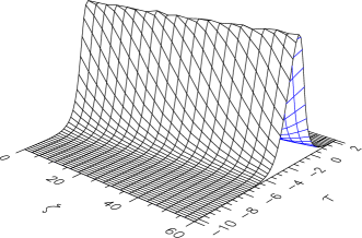
Figure 1: GFEA soliton propagation. This shows the pump field profile (i.e. $\left|A\right|^{2}$) for a $\Delta=3$ pulse with group/phase velocity ratio of $\sigma=1$. The pulse starts with an offset of $\tau_{0}=-5$.

Figure 2: GFEA soliton velocity shifts ($-\delta v$). as a function of bandwidth multiplier $\Delta$. The pulses at $\Delta=1$ are approximately 10 cycles long. The symbols represent the velocity shifts obtained by numerical simulation, the solid lines the corresponding theoretical prediction. The numerical labels give the group/phase velocity ratio $\sigma$ corresponding to the nearest data points.

II.2 Theoretical Group Velocity Shift

It is not necessary to rely on computer simulations to predict this few-cycle shift in the group velocity, at least in the case of weak few-cycle effects. Biswas & Aceves Biswas and Aceves (2001) have already provided a multi-scale method giving the effects of various perturbations on standard NLS soliton propagation. Their eqn.(13) applied to our NLS equation gives the velocity shift as

$$v_{A} = \frac{d}{dz}\frac{\int_{-\infty}^{+\infty}tA^{*}A~{}dt}{\int_{-\infty}^{+\infty}A^{*}A~{}dt},$$ (5)

which we can evaluate by inserting the SVEA soliton profile from eqn.(2) into the few-cycle perturbation term in eqn.(4), namely

$$R = \chi\left(2-\sigma\right)\partial_{t}A^{*}A^{2}/\omega_{0}.$$ (6)

This is of the same form as the $\lambda$ “self-steepening” term $\lambda\partial_{t}\left|q\right|^{2}q$ in Biswas & Aceves Biswas and Aceves (2001), allowing for the changed notation and different prefactors. Solving to first order in the perturbation and using the intermediate quantity   $\bar{\tau}=\int_{-\infty}^{+\infty}t\partial_{z}\left(A^{*}A\right)~{}dt$ gives

$$\bar{\tau} = -2\chi\frac{2-\sigma}{\omega_{0}}\eta^{4}\frac{\pi}{2\eta},$$ (7)

$$v_{A} = -\chi\frac{2-\sigma}{\omega_{0}}\eta^{2}.$$ (8)

With our parameters, this gives a velocity shift of

$$\delta v = v_{A}=-\frac{\left(2-\sigma\right)\Delta}{20\pi}\approx-0.01592\left(2-\sigma\right)\Delta.$$ (9)

Since we assume a small perturbation (eqn.(6)), it is clear that this prediction is most valid for higher carrier frequencies and/or weaker nonlinearities, i.e. where the effect of the nonlinearity is small over the time of an optical cycle.

The predictions of eqn.(9) are plotted as solid lines in fig. 2, and the agreement with the numerical simulations is seen to be remarkably good, even for very wideband pulses (e.g. the $\sim$1 cycle cases where $\Delta=8$). However, the effect of the higher order GFEA contributions, present in the simulations but not in eqn.(9), becomes visible near $\sigma=2$, where the first order corrections become small.

III Parametric Solitons

Parametric solitons, otherwise known as “simultons” or “quadratic solitons”, rely on the interplay between dispersion and a second order $\chi^{(2)}$ interaction to maintain fixed envelope profiles between a pair of pulses propagating in tandem.

If we modify the standard (dimensionless) propagation equation of Werner & DrummondWerner and Drummond (1993) to include few-cycle terms to first order, with carrier frequencies $\omega_{\psi}=2\omega_{\phi}$ and wavevectors $\beta_{0\psi}=2\beta_{0\phi}$, we get

$$\partial_{\xi}\psi+\frac{\imath\beta_{2\psi}}{2\left|\beta_{2\phi}\right|}\partial_{\tau}^{2}\psi = -\left[1+\imath\frac{2-\sigma}{\omega_{\psi}}\partial_{\tau}\right]\frac{\phi^{2}}{2},$$ (10)

$$\partial_{\xi}\phi+\frac{\imath}{2}{\textrm{ sgn}}(\beta_{2\phi})\partial_{\tau}^{2}\phi = \left[1+\imath\frac{2-\sigma}{\omega_{\phi}}\partial_{\tau}\right]\psi\phi^{*}.$$ (11)

Here $\beta_{1\psi},\beta_{1\phi}$ and $\beta_{2\psi},\beta_{2\phi}$ are the group velocities and group velocity dispersions respectively. We work in a co-moving frame where $\beta_{1\psi}=\beta_{1\phi}$, so the two pulses remain co-propagating. This ensures that their group-phase velocity ratios are identical ($\sigma=\sigma_{\psi}=\sigma_{\phi}$). Distance and times are normalised using $z_{0}^{-1}=\left|\chi\Phi_{0}\right|=\left|\beta_{2\phi}\right|/t_{0}^{2}$, and $\xi=z/z_{0}$, $\tau=t/t_{0}$.

In the SVEA limit ($\left|\partial_{\tau}\psi\right|/\omega_{\psi}\rightarrow 0$, and $\left|\partial_{\tau}\phi\right|/\omega_{\phi}\rightarrow 0$), the standard anzatz gives the solutions

$$\phi(z,t)=\Phi/\Psi_{0} = \phi_{0}{\textrm{ sech}}^{2}(\kappa\tau)\exp(\imath\theta_{\phi}\xi),$$ (12)

$$\psi(z,t)=\Psi/\Psi_{0} = \psi_{0}{\textrm{ sech}}^{2}(\kappa\tau)\exp(\imath\theta_{\psi}\xi),$$ (13)

where $\theta_{\phi}=2\kappa^{2}{\textrm{ sgn}}(\beta_{2\phi})$, $\theta_{\psi}+2\kappa^{2}\left(\beta_{2\psi}/\left|\beta_{2\phi}\right|\right)-z_{0}\left(\beta_{2\psi}-2\beta_{2\phi}\right)=0$ are time independent constants. In our chosen frame of reference, these parametric soliton pulses have a group velocity of zero in the SVEA limit.

III.1 GFEA Simulations

We use the same basic code as for the Kerr soliton simulations, with the different form of nonlinearity. We use the normalised units described after eqn.(11).

Fig. 3 shows a typical result for the propagation of a parametric soliton. As for the Kerr soliton, few-cycle effects modify the group velocity. Results for different soliton widths $\Delta$ and different $\sigma$ values are summarised in fig. 4. The velocity shift remains remarkably linear even for extremely wideband pulses. Note that $\Delta=5$ corresponds to a 2 cycle pulse, for which the electric field profile would not appear particularly ${\textrm{ sech}}^{2}$ shaped, because of the small number of carrier oscillations. In reality, however, the parabolic form of the material dispersion assumed in the simulations will not be maintained over such a wide bandwidth, and other distortions are likely to predominate over few-cycle effects in these circumstances. In addition, as the bandwidth increases, the spectra of the two pulses will eventually overlap, despite the separation of their carrier frequencies.

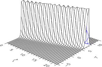
Figure 3: GFEA simulated simulton propagation: the pump field profile $\left|\psi\right|^{2}$ for a 3-cycle pulse ($\Delta=3$) with $\sigma=1$. The signal field profile $\left|\phi\right|^{2}$ is similar.

Figure 4: GFEA simulated simulton velocity shifts $-\delta v$ as a function of bandwidth multiplier $\Delta$. The pulses at $\Delta=1$ are approximately 10 cycles long. The symbols represent the velocity shifts obtained by numerical simulation, the solid lines the corresponding theoretical prediction. The numerical labels give the group/phase velocity ratio $\sigma$ corresponding to the nearest data points.

III.2 Theoretical Group Velocity Shift

As described in section II, we followed the method of Biswas and AcevesBiswas and Aceves (2001) to show how few-cycle corrections for NLS solitons would modify the group velocity. We now show that the same method can predict parametric soliton group velocity shifts. Eqn.(13) from Biswas and AcevesBiswas and Aceves (2001) applied to the equations for parametric solitons gives the velocity shifts as

$$v_{\phi} = \frac{d}{d\xi}\frac{\int_{-\infty}^{+\infty}\tau\phi^{*}\phi~{}d\tau}{\int_{-\infty}^{+\infty}\phi^{*}\phi~{}d\tau},$$ (14)

$$v_{\psi} = \frac{d}{d\xi}\frac{\int_{-\infty}^{+\infty}\tau\psi^{*}\psi~{}d\tau}{\int_{-\infty}^{+\infty}\psi^{*}\psi~{}d\tau},$$ (15)

which we can evaluate by inserting the SVEA soliton profiles (from eqn.(12) and (13)) along with the few-cycle perturbations to the propagation:

$$R_{\phi} = \left(2-\sigma\right)\partial_{\tau}\psi\phi^{*}/\omega_{\psi},$$ (16)

$$R_{\psi} = -\left(2-\sigma\right)\partial_{\tau}\phi^{2}/\left(2\omega_{\psi}\right).$$ (17)

Solving to first order in the perturbation(s) and using the intermediate quantity   $\bar{\tau}_{\phi}=\int_{-\infty}^{+\infty}\tau\partial_{\xi}\left(\phi^{*}\phi\right)~{}d\tau$ gives

$$\bar{\tau}_{\phi} = \frac{2-\sigma}{\omega_{\phi}}\left(\psi_{0}\phi_{0}^{*}\phi_{0}+\psi_{0}^{*}\phi_{0}\phi_{0}^{*}\right)\frac{-16\pi}{45},$$ (18)

$$v_{\phi} = -\frac{8}{15}\frac{2-\sigma}{\omega_{\phi}}\left(\psi_{0}+\psi_{0}^{*}\right),$$ (19)

and similarly using   $\bar{\tau}_{\psi}=\int_{-\infty}^{+\infty}\tau\partial_{\xi}\left(\psi^{*}\psi\right)~{}d\tau$,

$$\bar{\tau}_{\psi} = -\frac{1}{2}\frac{2-\sigma}{\omega_{\psi}}\left({\phi_{0}^{*}}^{2}\psi_{0}+\phi_{0}^{2}\psi_{0}^{*}\right)\frac{-16\pi}{45},$$ (20)

$$v_{\psi} = \frac{4}{15}\frac{2-\sigma}{\omega_{\psi}}\left({\phi_{0}^{*}}^{2}/\psi_{0}^{*}+\phi_{0}^{2}/\psi_{0}\right).$$ (21)

In our numerical simulations we used $\psi_{0}=3$, $\phi_{0}=-6\imath$, and $\omega_{\psi}=2\omega_{\phi}=20\pi/\Delta$, so that

$$\delta v = v_{\psi}~{}=~{}v_{\phi}\approx-0.1019\left(2-\sigma\right)\Delta.$$ (22)

Because the velocity shift for each pulse of the pair making up the parametric soliton is the same (at least for first order GFEA corrections), the two pulses remain co-propagating, and the soliton survives.

The predictions of eqn.(22) are plotted as solid lines in fig. 4, and the agreement with the numerical simulations is seen to be remarkably good, even for wideband pulses (e.g. $\Delta\geq 4$). However, the effect of the higher order GFEA contributions, present in the simulations but not in eqn.(22), start to become visible above $\sigma\approx 1.60$, since near $\sigma=2$ the first order few-cycle correction does not dominate.

IV Conclusion

We have investigated two types of soliton propagation beyond the standard SVEA regime both theoretically and numerically. The most important result is that, according to the GFEA theory, soliton propagation remains robust in the few-cycle regime. This is obviously encouraging for proposed applications involving ultrashort solitons – although for such wideband pulses, there are other complications beyond just the few-cycle ones examined in this paper.

The major effect of the shortening pulses is a group velocity shift, despite the fact that the perturbation term does not look like a a simple group-velocity term. It is likely that the few-cycle “phase twist” added to the propagation also affects the other properties of soliton pulses, e.g. collisions, which has obvious potential implications for soliton-based ultrafast optical logic gates.

References

- Trillo et al. (1988) S. Trillo, S. Wabnitz, E. M. Wright, and G. I. Stegeman, Optics Letters 13, 672 (1988),
- Potasek (1989) M. J. Potasek, J. Appl. Phys. 65, 941 (1989),
- Drummond et al. (1994) P. D. Drummond, J. Breslin, W. Man, and R. M. Shelby, Springer Proceedings in Physics 77, 194 (1994).
- Gromov and Talanov (2000) E. M. Gromov and V. I. Talanov, Chaos 10, 551 (2000),
- Zaspel et al. (2001) C. E. Zaspel, J. H. Mantha, Y. G. Rapoport, and V. V. Grimalsky, Phys. Rev. B 64, 064416 (2001),
- Kinsler and New (2003) P. Kinsler and G. H. C. New, Phys. Rev. A 67, 023813 (2003),
- Kinsler (2002) P. Kinsler, arXiv.org physics, 0212014 (2002),
- Zaspel (1999) C. E. Zaspel, Phys. Rev. Lett. 82, 723 (1999), but see also Park and Han (2000),
- Park and Han (2000) Q. Han Park and S. H. Han, Phys. Rev. Lett. 84, 3732 (2000),
- Biswas and Aceves (2001) A. Biswas and A. B. Aceves, J. Mod. Opt. 48, 1135 (2001),
- Agrawal (1995) G. P. Agrawal, Nonlinear Fiber Optics (Academic Press, 1995).
- Wabnitz et al. (1995) S. Wabnitz, Y. Kodama, and A. B. Aceves, Opt. Fiber Technol. 41, 187 (1995),
- Brabec and Krausz (1997) T. Brabec and F. Krausz, Phys. Rev. Lett. 78, 3282 (1997),
- Trippenbach et al. (2002) M. Trippenbach, W. Wasilewski, P. Kruk, G. Bryant, G. Fibich, and Y. Band, Opt. Comm. 210, 385 (2002),
- Werner and Drummond (1993) M. Werner and P. Drummond, JOSA B 10, 2394 (1993),