A linear theory for control of non-linear stochastic systems

Abstract

We address the role of noise and the issue of efficient computation in stochastic optimal control problems. We consider a class of non-linear control problems that can be formulated as a path integral and where the noise plays the role of temperature. The path integral displays symmetry breaking and there exist a critical noise value that separates regimes where optimal control yields qualitatively different solutions. The path integral can be computed efficiently by Monte Carlo integration or by Laplace approximation, and can therefore be used to solve high dimensional stochastic control problems.

Optimal control of non-linear systems in the presence of noise is a very general problem that occurs in many areas of science and engineering. It underlies autonomous system behavior, such as the control of movement and planning of actions of animals and robots, but also for instance the optimization of financial investment policies and control of chemical plants. The problem is simply stated: given that the system is in this configuration at this time, what is the optimal course of action to reach a goal state at some future time. The cost of each time course of actions consists typically of a path contribution, that specifies the amount of work or other cost of the trajectory, and an end cost, that specifies to what extend the trajectory reaches the goal state.

In the absence of noise, the optimal control problem can be solved in two ways: using the Pontryagin Minimum Principle (PMP) Pontryagin et al. (1962) which is a pair of ordinary differential equations that are similar to the Hamilton equations of motion or using the Hamilton-Jacobi-Bellman (HJB) equation, which is a partial differential equation Bellman and Kalaba (1964).

In the presence of (Wiener) noise, the PMP formalism is replaced by a set of stochastic differential equations which become difficult to solve (see however Yong and Zhou (1999)). The inclusion of noise in the HJB framework is mathematically quite straight-forward, yielding the so-called stochastic HJB equation Stengel (1993). Its solution , however, requires a discretization of space and time and the computation becomes intractable in both memory requirement and CPU time in high dimensions. As a result, deterministic control can be computed efficiently using the PMP approach, but stochastic control is intractable due to the curse of dimensionality.

For small noise, one expects that optimal stochastic control resembles optimal deterministic control, but for larger noise, the optimal stochastic control can be entirely different from the deterministic control Russell and Norvig (2003), but there is currently no good understanding how noise affects optimal control.

In this paper, we address both the issue of efficient computation and the role of noise in stochastic optimal control. We consider a class of non-linear stochastic control problems, that can be formulated as a statistical mechanics problem. This class of control problems includes arbitrary dynamical systems, but with a limited control mechanism. It contains linear-quadratic Stengel (1993) control as a special case. We show that under certain conditions on the noise, the HJB equation can be written as a linear partial differential equation

$$-\partial_{t}\psi=H\psi$$ (1)

with $H$ a (non-Hermitian) operator. Eq. 1 must be solved subject to a boundary condition at the end time. As a result of the linearity of Eq. 1, the solution can be obtained in terms of a diffusion process evolving forward in time, and can be written as a path integral. The path integral has a direct interpretation as a free energy, where noise plays the role of temperature.

This link between stochastic optimal control and a free energy has two immediate consequences. 1) Phenomena that allow for a free energy description, typically display phase transitions. We argue that for stochastic optimal control one can identify a critical noise value that separates regimes where the optimal control is qualitatively different and illustrate this with a simple example. 2) Since the path integral appears in other branches of physics, such as statistical mechanics and quantum mechanics, we can borrow approximation methods from those fields to compute the optimal control approximately. We show how the Laplace approximation can be combined with Monte Carlo sampling to efficiently compute the optimal control.

Let $\vec{x}$ be an $n$-dimensional stochastic variable that is subject to the stochastic differential equation

$$d\vec{x}=(\vec{b}(\vec{x},t)+\vec{u})dt+d\vec{\xi}$$ (2)

with $d\vec{\xi}$ a Wiener process with $\left<d\xi_{i}d\xi_{j}\right>=\nu_{ij}dt$, and $\nu_{ij}$ independent of $\vec{x},\vec{u},t$. $\vec{b}(\vec{x},t)$ is an arbitrary $n$-dimensional function of $\vec{x}$ and $t$, and $\vec{u}$ an $n$-dimensional vector of control variables. Given $\vec{x}$ at an initial time $t$, the stochastic optimal control problem is to find the control path $\vec{u}(\cdot)$ that minimizes

$$C(\vec{x},t,\vec{u}(\cdot))=$$

$$\left<\phi(\vec{x}(t_{f}))+\int_{t}^{t_{f}}d\tau\left(\frac{1}{2}\vec{u}(\tau)^{T}{\bf R}\vec{u}(\tau)+V(\vec{x}(\tau),\tau)\right)\right>_{\vec{x}}$$

(3)

with ${\bf R}$ a matrix, $V(\vec{x},t)$ a time-dependent potential, and $\phi(\vec{x})$ the end cost. The brackets $\left<\right>_{\vec{x}}$ denote expectation value with respect to the stochastic trajectories (2) that start at $\vec{x}$.

One defines the optimal cost-to-go function from any time $t$ and state $\vec{x}$ as

$$J(\vec{x},t) = \min_{\vec{u}(\cdot)}C(\vec{x},t,\vec{u}(\cdot)).$$ (4)

$J$ satisfies the stochastic HJB equation which takes the form

$$-\partial_{t}J = \min_{\vec{u}}\left(\frac{1}{2}\vec{u}^{T}{\bf R}\vec{u}+V+(\vec{b}+\vec{u})^{T}\vec{\nabla}J+\frac{1}{2}\mathrm{Tr}\left({\bm{\nu}}{\bm{\nabla}}^{2}J\right)\right)$$

$$= -\frac{1}{2}(\vec{\nabla}J)^{T}{\bf R}^{-1}\vec{\nabla}J+V+\vec{b}^{T}\vec{\nabla}J+\frac{1}{2}\mathrm{Tr}\left({\bm{\nu}}{\bm{\nabla}}^{2}J\right)$$

with $\mathrm{Tr}({\bm{\nu}}{\bm{\nabla}}^{2}J)=\sum_{ij}\nu_{ij}\partial^{2}J/\partial x_{i}\partial x_{j}$ and

$$\vec{u}=-{\bf R}^{-1}\vec{\nabla}J(\vec{x},t)$$ (6)

the optimal control at $\vec{x},t$. The HJB equation is non-linear in $J$ and must be solved with end boundary condition $J(\vec{x},t_{f})=\phi(\vec{x})$.

Define $\psi(\vec{x},t)$ through

$$J(\vec{x},t)=-\lambda\log\psi(\vec{x},t)$$ (7)

and assume there exists a scalar $\lambda$ such that

$$\lambda\delta_{ij}=({\bf R}{\bm{\nu}})_{ij}$$ (8)

with $\delta_{ij}$ the Kronecker delta. In the one dimensional case, such a $\lambda$ can always be found. In the higher dimensional case, this restricts the matrices ${\bf R}\propto{\bm{\nu}}^{-1}$ . Eq. 8 reduces the dependence of optimal control on the $n$-dimensional noise matrix to a scalar value $\lambda$ that will play the role of temperature. Eq. LABEL:hjb reduces to the linear equation 1 with

$$H = -\frac{V}{\lambda}+\vec{b}^{T}\vec{\nabla}+\frac{1}{2}\mathrm{Tr}({\bm{\nu}}{\bm{\nabla}}^{2})$$ (9)

Let $\rho(\vec{y},\tau|\vec{x},t)$ with $\rho(\vec{y},t|\vec{x},t)=\delta(\vec{y}-\vec{x})$ describe a diffusion process for $\tau>t$ defined by the Fokker-Planck equation

$$\partial_{\tau}\rho=H^{\dagger}\rho=-\frac{V}{\lambda}\rho-\vec{\nabla}^{T}(\vec{b}\rho)+\frac{1}{2}\mathrm{Tr}({\bm{\nu}}{\bm{\nabla}}^{2})\rho$$ (10)

with $H^{\dagger}$ the Hermitian conjugate of $H$. Then $A(\tau)=\int d\vec{y}\rho(\vec{y},\tau|\vec{x},t)\psi(\vec{y},\tau)$ is independent of $\tau$ and in particular $A(t)=A(t_{f})$. It immediately follows that

$$\psi(\vec{x},t) = \int d\vec{y}\rho(\vec{y},t_{f}|\vec{x},t)\exp(-\phi(\vec{y})/\lambda)$$ (11)

We arrive at the important conclusion that $\psi(\vec{x},t)$ can be computed either by backward integration using Eq. 1 or by forward integration of a diffusion process given by Eq. 10.

We can write the integral in Eq. 11 as a path integral. We use the standard argument Kleinert (1995) and divide the time interval $t\rightarrow t_{f}$ in $n_{1}$ intervals and write $\rho(\vec{y},t_{f}|\vec{x},t)=\prod_{i=1}^{n_{1}}\rho(\vec{x}_{i},t_{i}|\vec{x}_{i-1},t_{i-1})$ and let $n_{1}\rightarrow\infty$. The result is

$$\psi(\vec{x},t) = \int[d\vec{x}]_{\vec{x}}\exp\left(-\frac{1}{\lambda}S(\vec{x}(t\rightarrow t_{f}))\right)$$ (12)

with $\int[d\vec{x}]_{\vec{x}}$ an integral over all paths $\vec{x}(t\rightarrow t_{f})$ that start at $\vec{x}$ and with

$$S(\vec{x}(t\rightarrow t_{f})) = \phi(\vec{x}(t_{f})+\int_{t}^{t_{f}}d\tau\left(\frac{1}{2}\left(\frac{d\vec{x}(\tau)}{d\tau}-\vec{b}(\vec{x}(\tau),\tau)\right)^{T}{\bf R}\left(\frac{d\vec{x}(\tau)}{d\tau}-\vec{b}(\vec{x}(\tau),\tau)\right)+V(\vec{x}(\tau),\tau)\right)$$ (13)

the Action associated with a path. From Eqs. 7 and 12, the cost-to-go $J(x,t)$ becomes a log partition sum (ie. a free energy) with temperature $\lambda$.

The path integral Eq. 12 can be estimated by stochastic integration from $t$ to $t_{f}$ of the diffusion process Eq. 10 in which particles get annihilated at a rate $V(\vec{x},t)/\lambda$:

$$\vec{x} = \vec{x}+\vec{b}(\vec{x},t)dt+d\vec{\xi},\quad\mbox{with probability}~{}1-Vdt/\lambda$$

$$\vec{x} = \dagger,\quad\mbox{with probability}~{}Vdt/\lambda$$ (14)

where $\dagger$ denotes that the particle is taken out of the simulation. Denote the trajectories by $\vec{x}_{\alpha}(t\rightarrow t_{f}),\alpha=1,\ldots,N$. Then, $\psi(\vec{x},t)$ and $\vec{u}$ are estimated as

$$\hat{\psi}(\vec{x},t) = \sum_{\alpha\in\mathrm{alive}}w_{\alpha}$$ (15)

$$\hat{\vec{u}}dt = \frac{1}{\hat{\psi}(\vec{x},t)}\sum_{\alpha\in\mathrm{alive}}^{N}w_{\alpha}d\vec{\xi}_{\alpha}(t)$$ (16)

$$w_{\alpha} = \frac{1}{N}\exp(-\phi(\vec{x}_{\alpha}(t_{f}))/\lambda)$$

where ’alive’ denotes the subset of trajectories that do not get killed along the way by the $\dagger$ operation. The normalization $1/N$ ensures that the annihilation process is properly taken into account. Eq. 16 states that optimal control at time $t$ is obtained by averaging the initial directions of the noise component of the trajectories $d\vec{\xi}_{\alpha}(t)$, weighted by their success at $t_{f}$.

The above sampling procedure can be quite inefficient, when many trajectories get annihilated. One of the simplest procedures to improve it is by importance sampling. We replace the diffusion process that yields $\rho(\vec{y},t_{f}|\vec{x},t)$ by another diffusion process, that will yield $\rho^{\prime}(\vec{y},t_{f}|\vec{x},t)=\exp(-S^{\prime}/\lambda)$. Then Eq. 12 becomes,

$$\psi(\vec{x},t) = \int[d\vec{x}]_{\vec{x}}\exp\left(-S^{\prime}/\lambda\right)\exp\left(-(S-S^{\prime})/\lambda\right)$$

The idea is to chose $\rho^{\prime}$ such as to make the sampling of the path integral as efficient as possible. Here, we use the Laplace approximation, which is given by the $k$ deterministic trajectories $x_{\beta}(t\rightarrow t_{f})$ that minimize the Action

$$J(\vec{x},t) \approx -\lambda\log\sum_{\beta=1}^{k}\exp(-S(\vec{x}_{\beta}(t\rightarrow t_{f})/\lambda)$$ (17)

The Laplace approximation ignores all fluctuations around the modes and becomes exact in the limit $\lambda\rightarrow 0$. The Laplace approximation can be computed efficiently, requiring ${\cal O}(n^{2}m^{2})$ operations, where $m$ is the number of time discretization.

For each Laplace trajectory, we define a diffusion processes $\rho^{\prime}_{\beta}$ according to Eq. 14 with $\vec{b}(\vec{x},t)=\dot{\vec{x}}_{\beta}(t)$. The estimators for $\psi$ and $\vec{u}$ are given again by Eqs. 15 and 16, but with weights

$$w_{\alpha} = \frac{1}{N}\exp\left(-\left(S(\vec{x}_{\alpha}(t\rightarrow t_{f}))-S^{\prime}_{\beta}(\vec{x}_{\alpha}(t\rightarrow t_{f}))\right)/\lambda\right).$$

$S$ is the original Action Eq. 13 and $S^{\prime}_{\beta}$ is the new Action for the Laplace guided diffusion. When there are multiple Laplace trajectories one should include all of these in the sample.

We give a simple one-dimensional example of a double slit to illustrate the effectiveness of the Laplace guided MC method and to show how the optimal cost-to-go undergoes symmetry breaking as a function of the noise.

Consider a stochastic particle that moves with constant velocity from $t=0$ to $t_{f}=2$ in the horizontal direction and where there is deflecting noise in the $x$ direction:

$$dx = udt+d\xi$$

The cost is given by Eq. 3 with $\phi(x)=\frac{1}{2}x^{2}$ and $V(x,t_{1})$ implements a slit at an intermediate time $t_{1}=1$ (Fig. 1). Solving the cost-to-go by means of the forward computation using Eq. 11 can be done in closed form. The exact result, the Laplace approximation Eq. 17 and the Laplace guided importance sampling result using Eq. LABEL:importance_weights are plotted for $t=0$ as a function of $x$ in Fig. 2. For each $x$, the Laplace approximation consists of the two deterministic trajectories, each being piecewise linear, starting at $t=0$ in $x$ and ending at $t=2$ in $x=0$.

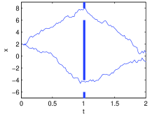
Figure 1: A double slit is placed at $t=1$ with openings at $-6<x<-4$ and $6<x<8$. $V=\infty$ for $t=1$ outside the openings, and zero otherwise. Also shown are two example trajectories under optimal control.

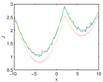
Figure 2: Comparison of Laplace approximation (dotted line) and Monte Carlo importance sampling (solid jagged line) of $J(x,t=0)$ with exact result (solid smooth line) for the double slit problem. The importance sampler used $N=100$ trajectories for each $x$. $R=0.1,\nu=1,dt=0.02$.

We see that the Laplace approximation is quite good for this example, in particular when one takes into account that a constant shift in $J$ does not affect the optimal control. The MC importance sampler has maximal error of order 0.1 and is significantly better than the Laplace approximation. Naive MC sampling using Eq. 14 (not shown) fails for this problem, because most trajectories get killed by the infinite potential. Numerical simulations using $N=100000$ trajectories yield estimation errors in $J$ up to approximately 6 for certain values of $x$.

We show an example how optimal stochastic control exhibits spontaneous symmetry breaking. For two slits of width $\epsilon$ at $x=\pm 1$, the cost-to-go becomes to lowest order in $\epsilon$:

$$J(x,t) = \frac{R}{T}\left(\frac{1}{2}x^{2}-\nu T\log 2\cosh\frac{x}{\nu T}\right)+\mathrm{const.},\quad t<t_{1}$$

where the constant diverges as ${\cal O}(\log\epsilon)$ independent of $x$ and $T=t_{1}-t$ the time to reach the slits. The expression between brackets is a typical free energy with inverse temperature $\beta=1/\nu T$. It displays a symmetry breaking at $\nu T=1$. The optimal control is given by the gradient of $J$:

$$u=\frac{1}{T}\left(\tanh\frac{x}{\nu T}-x\right)$$ (19)

For $T>1/\nu$ (far in the past) optimal control steers towards $x=0$ (between the targets) and delays the choice which slit to aim for until later. The reason why this is optimal is that the expected diffusion alone of size $\sqrt{\nu T}$ is likely to reach any of the slits without control (although it is not clear yet which slit). Only sufficiently late in time ($T<1/\nu$) should one make a choice.

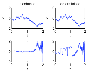
Figure 3: Symmetry breaking in $J$ as a function of $T$ implies a ’delayed choice’ mechanism for optimal stochastic control. When the target is far in the future, the optimal policy is to steer between the targets. Only when $T<1/\nu$ should one aim for one of the targets. Sample trajectories (top row) and controls (bottom row) under stochastic control (left column) and deterministic control (right column). $\nu=R=1$, $t_{1}=2$.

Figure 3 depicts two trajectories and their controls under stochastic optimal control (Eq. 19) and deterministic optimal control (Eq. 19 with $\nu=0$), using the same realization of the noise. Note, that at early times the deterministic control drives $x$ away from zero whereas in the stochastic control drives $x$ towards zero and is smaller in size. The stochastic control delays the choice for which slit to aim until $T\approx 1$.

In summary, we have shown that stochastic optimal control involves symmetry breaking with qualitatively different solutions for high and low noise levels. This property is expected to be true also for more general stochastic control problems. The path integral formulation allows for an efficient solution of the HJB equation because it replaces the intractable $n$-dimensional numerical integration by a Monte Carlo sampling, which is known to be often much more efficient. This approach will thus be of direct practical value for the control of high dimensional, strongly non-linear, systems, such as for instance robot arms, navigation of autonomous systems, and chemical reactions. For realistic applications, naive sampling should be replaced by more advanced sampling schemes, such as importance sampling or a Metropolis method, and should be combined with efficient discretization such as splines, wavelets or a Fourier basis Miller (1975); Freeman and Doll (1984).