Constraints on the Size of the Smallest Triggering Earthquake from the ETAS Model, Båth’s Law, and Observed Aftershock Sequences

Abstract

The physics of earthquake triggering together with simple assumptions of self-similarity impose the existence of a minimum magnitude $m_{0}$ below which earthquakes do not trigger other earthquakes. Noting that the magnitude $m_{d}$ of completeness of seismic catalogs has no reason to be the same as the magnitude $m_{0}$ of the smallest triggering earthquake, we use quantitative fits and maximum likelihood inversions of observed aftershock sequences as well as Båth’s law, compare with ETAS model predictions and thereby constrain the value of $m_{0}$. We show that the branching ratio $n$ (average number of triggered earthquake per earthquake also equal to the fraction of aftershocks in seismic catalogs) is the key parameter controlling the minimum triggering magnitude $m_{0}$. Conversely, physical upper bounds for $m_{0}$ derived from state- and velocity-weakening friction indicate that at least 60 to 70 percent of all earthquakes are aftershocks.

SORNETTE and WERNER CONSTRAINTS ON THE SMALLEST TRIGGERING EARTHQUAKE D. Sornette, Department of Earth and Space Sciences, and Institute of Geophysics and Planetary Physics, University of California, Los Angeles, California 90095, USA and Laboratoire de Physique de la Matière Condensée, CNRS UMR6622, Université de Nice-Sophia Antipolis, Parc Valrose, 06108 Nice Cedex 2, France. (sornette@moho.ess.ucla.edu) M. J. Werner, Department of Earth and Space Sciences, and Institute of Geophysics and Planetary Physics, University of California, Los Angeles, California 90095, USA. (werner@moho.ess.ucla.edu)

Gindraft=false

1 Introduction

Scale invariance in earthquake phenomena is widely manifested empirically, in the magnitude-frequency Gutenberg-Richter relation, in the aftershock Omori decay rate, and in many other relationships. Scale-invariance means that there are no prefered length scales in seismogenic processes and in spatio-temporal structures. However, there are many reports that purport to identify characteristic scales. As emphasized by Matsu’ura [1999], Aki [2000], and Sornette [2002], the search for characteristic structures in specific fault zones could allow the separation of large earthquakes from small ones and thus advance earthquake prediction.

Although there is clear evidence of deviations from self-similarity at large scales [Kagan, 1999; Pisarenko and Sornette, 2003], the issue is much murkier at small scales. For instance, Iio [1991], reports a lower magnitude cutoff $m_{\rm min}\approx-1.4$ for very small aftershocks of the 1984 Western Nagano Prefecture, Japan, earthquake ($m_{\rm JMA}=6.8$) in spite of the fact that the high sensitivity of the observation system (focal distances less than $1$ km and very low ground noise) would have permitted to detect much smaller magnitudes. Based on induced seismicity associated with deep gold mines, Richardson and Jordan [1985] find a lower magnitude cutoff $m_{\rm min}\approx 0$ for friction-dominated earthquakes, while fracture-dominated earthquakes have no lower cutoff but an upper cut-off of magnitude $\approx 1$. Using deep borehole recordings, Abercrombie [1995a; 1995b] found that small earthquakes exist down to at least magnitude $0$ and that source scaling relationships hold down to at least $-1$. Based on seismic power spectra, on the evidence of a low-velocity low-Q zone reaching the top of the ductile part of the crust and on seismic guided waves in fault zones, Li et al. [1994] argue for a characteristic earthquake magnitude of about $3$ associated with the width of fault zones. Another characteristic magnitude in the range $4-5$ is proposed by Aki [1996], based on the simultaneous change of coda $Q^{-1}$ and the fractional rate of occurrence of earthquakes in this magnitude interval. The existence of a discrete hierarchy of scales has in addition been suggested by Sornette and Sammis [1995] based on the analysis of accelerated seismicity prior to large earthquakes and recently by Pisarenko et al. [2004] by using a non-parametric measure of deviations from power laws applied to the magnitude-frequency distributions of earthquakes in subduction zones. Evidence of a hierarchy of scales is also found in fragmentation and rupture processes [Sadovskii, 1999; Geilikman and Pisarenko, 1989; Sahimi and Arbabi, 1996; Ouillon et al., 1996; Johanson and Sornette, 1998; Suteanu, 2000].

From a theoretical point of view, the equation of motion for a continuum solid is scale-independent, suggesting that deformation processes in solids should produce self-similar patterns manifested in power law statistics. However, the symmetry of the equation does not warrant that the solutions of this equation share the same symmetry. Actually, the difference (when it exists) in the symmetry between a solution and its governing equation is known as the phenomenon of “spontaneous symmetry breaking” [Consoli and Stevenson, 2000] underlying a large variety of systems (for instance explaining the non-zero masses of fundamental particles [Englert, 2004]). Of course, length scales associated with rheology and existing structures can produce deviations from exact self-similarity. For instance, a transition from stable creep to a dynamic instability at a nucleation size whose dimensions depend on frictional and elastic parameters defines a minimum earthquake size [Dieterich, 1992], estimated at magnitude $\approx-3$ by Ben-Zion [2003]. This minimum size corresponds only to events triggered according to the mechanism of unstable sliding controlled by slip weakening and thus concerns friction-dominated earthquakes.

A different perspective is offered by models of triggered seismicity in which earthquakes (so-called foreshocks and mainshocks) trigger other earthquakes (so-called mainshocks and aftershocks, respectively). Recent studies suggest that maybe more than 2/3 of events are triggered by previous earthquakes (see Helmstetter and Sornette [2003b] and references therein). In this context, the relevant question is no more how small is the smallest earthquake but how small is the smallest earthquake which can trigger other earthquakes (and, in particular, larger earthquakes).

2 The ETAS model and the smallest triggering earthquake

To make this discussion precise, let us consider the epidemic-type aftershock sequence (ETAS) model, in which any earthquake may trigger other earthquakes, which in turn may trigger more, and so on. Introduced in slightly different forms by Kagan and Knopoff [1981] and Ogata [1988], the model describes statistically the spatio-temporal clustering of seismicity.

The ETAS model consists of three assumed laws about the nature of seismicity viewed as a marked point-process. We restrict this study to the temporal domain only, summing over the whole spatial domain of interest. First, the magnitude of any earthquake, regardless of time, space or magnitude of the mother shock, is drawn randomly from the exponential Gutenberg-Richter (GR) law. Its normalized probability density function (pdf) is expressed as

$$P(m)={b\ln(10)10^{-bm}\over 10^{-bm_{0}}-10^{-bm_{max}}},~{}~{}~{}~{}~{}m_{0}\leq m\leq m_{max},$$ (1)

where the exponent $b$ is typically close to one, and the cut-offs $m_{0}$ (see below) and $m_{max}$ serve to normalize the pdf. The upper cut-off $m_{max}$ is introduced to avoid unphysical, infinitely large earthquakes. Its value was estimated to be in the range $8-9.5$ [Kagan, 1999]. As the impact of a finite $m_{max}$ is quite weak in the calculations below, replacing the abrupt cut-off $m_{max}$ by a smooth taper would introduce negligible corrections to our results.

Second, the model assumes that direct aftershocks are distributed in time according to the modified “direct” Omori law (see Utsu et al. [1995] and references therein). Assuming $\theta>0$, the normalized pdf of the Omori law can be written as

$$\Psi(t)={\theta c^{\theta}\over(t+c)^{1+\theta}}.$$ (2)

Third, the number of direct aftershocks of an event of magnitude $m$ is assumed to follow the productivity law:

$$\rho(m)=k~{}10^{\alpha(m-m_{0})},~{}~{}~{}~{}~{}m_{0}\leq m\leq m_{max}.$$ (3)

Note that the productivity law (3) is zero below the cut-off $m_{0}$, i.e. earthquakes smaller than $m_{0}$ do not trigger other earthquakes, as is typically assumed in studies using the ETAS model. The existence of the small-magnitude cut-off $m_{0}$ is necessary to ensure the convergence of the models of triggered seismicity (in statistical physics of phase transitions and in particle physics, this is called an “ultra-violet” cut-off which is often necessary to make the theory convergent). Below, we show that there are observable consequences of the existence of the cut-off $m_{0}$ thus providing constraints on its physical value.

The key parameter of the model is defined as the number $n$ of direct aftershocks per earthquake, averaged over all magnitudes. Here, we must distinguish between the two cases $\alpha=b$ and $\alpha\neq b$:

$$n \equiv\int\limits_{m_{0}}^{m_{max}}P(m)\rho(m)dm$$ (6)

$$=\left\{\begin{array}[]{r@{\quad\quad}l}{kb\over b-\alpha}({1-10^{-(b-\alpha)(m_{max}-m_{0})}\over 1-10^{-b(m_{max}-m_{0})}}),&\alpha\neq b\\ {kb\ln(10)(m_{max}-m_{0})\over 1-10^{-b(m_{max}-m_{0})}},&\alpha=b.\end{array}\right.$$

Three regimes can be distinguished based on the value of $n$. The case $n<1$ corresponds to the subcritical regime, where aftershock sequences die out with probability one. The case $n>1$ describes unbounded, explosive seismicity that may lead to finite time singularities [Sornette and Helmstetter, 2002]. The critical case $n=1$ separates the two regimes.

The fact that we use the same cut-off for the productivity cut-off and the Gutenberg-Richter (GR) cut-off is not a restriction as long as the real cut-off for the Gutenberg-Richter law is smaller than or equal to the cut-off for the productivity law. In that case, truncating the GR law at the productivity cut-off just means that all smaller earthquakes, which do not trigger any events, do not participate in the cascade of triggered events. This should not be confused with the standard incorrect procedure in many previous studies of triggered seismicity of simply replacing the GR and productivity cut-off $m_{0}$ with the detection threshold $m_{d}$ in equations (1) and (3) (see, for example, Ogata [1988]; Zhuang et al. [2004]; Helmstetter and Sornette [2002]; Console et al. [2003]; Ogata [1998]; Felzer et al. [2002]; Kagan [1991]). This may lead to a bias in the estimated parameters.

The realization that the detection threshold $m_{d}$ and the triggering threshold $m_{0}$ are different leads to the question of whether we can extract the size of the smallest triggering earthquake. Here, we infer useful information on $m_{0}$ from the physics of earthquake triggering embodied in the simple ETAS formalism, from Båth’s law and from available catalogs.

There is no loss of generality in considering one (independent) branch (sequence or cascade of aftershocks) of the ETAS model. Let an independent background event of magnitude $M_{1}$ occur at some origin of time. The mainshock will trigger direct aftershocks according to the productivity law (3). Each of the direct aftershocks will trigger their own aftershocks, which in turn produce their own, and so on. Averaged over all magnitudes, each aftershock produces $n$ direct offspring according to (6). Thus, in infinite time, we can write the average of the total number $N_{total}$ of direct and indirect aftershocks of the initial mainshock as an infinite sum over terms of (3) multiplied by $n$ to the power of the generation [Helmstetter et al., 2004], which can be expressed for $n<1$ as:

$$N_{total} =\rho(M_{1})+\rho(M_{1})n+\rho(M_{1})n^{2}+...$$ (7)

$$={k~{}10^{\alpha(M_{1}-m_{0})}\over 1-n}$$

However, since we can only detect events above the detection threshold $m_{d}$, the total number of observed aftershocks $N_{obs}$ of the sequence is simply $N_{total}$ multiplied by the fraction of events above the detection threshold, given by $(10^{-b(m_{max}-m_{d})}-1)(10^{-b(m_{max}-m_{d})}-1)^{-1}$ according to the GR distribution. The observed number of events in the sequence is therefore

$$N_{obs} = N_{total}~{}\left({10^{b(m_{max}-m_{d})}-1\over 10^{b(m_{max}-m_{0})}-1}\right)$$ (8)

$$= {k~{}~{}10^{\alpha(M_{1}-m_{0})}\over 1-n}~{}\left({10^{b(m_{max}-m_{d})}-1\over 10^{b(m_{max}-m_{0})}-1}\right)~{}.$$

Equation (8) predicts the average observed number of direct and indirect aftershocks of a mainshock of magnitude $M_{1}>m_{d}$. To estimate $m_{0}$, we need to eliminate or find estimates of the three unknowns $n$, $k$, and $N_{obs}$. We can eliminate $k$ through the expression (6) for $n$, leaving $n$ and $N_{obs}$. The mean number of observed aftershocks as a function of mainshock magnitude $M_{1}$ was estimated by Helmstetter et al. [2004] and Felzer et al. [2003] and can also be obtained from Båth’s law. In the following sections, we use these three estimates for $N_{obs}$ and thus obtain $m_{0}$ as a function of the only remaining unknown $n$. Acknowledging the controversy surrounding the estimation of the percentage of aftershocks in a catalog, we nevertheless use existing estimates of $n$ to finally obtain quantitative values for $m_{0}$.

3 Constraint on the smallest triggering earthquake from the ETAS model and observed estimates of aftershock numbers

Following the recipe outlined above, we begin by using the estimates of the observed number of aftershocks $N_{obs}$ obtained by Helmstetter et al. [2004] in order to find $m_{0}$ as a function of $n$. Helmstetter et al. [2004] sidestepped the problems associated with maximum likelihood estimates of the complete model parameters by fitting stacked observed aftershock rates within pre-defined space-time windows using the formula

$$\lambda_{fit}(t)={K_{fit}~{}~{}10^{\alpha M_{1}-bm_{d}}\over t^{p_{fit}}}~{},$$ (9)

based on scaling laws (the GR law, the Omori law, and the productivity law) discussed above. The constant $K_{fit}$ includes all aftershocks, direct and indirect, and thus corresponds to a global renormalized constant different from $k$ in the ETAS productivity law (3). Furthermore, $p_{fit}$ is also a global exponent, which may be different from the local exponent $1+\theta$ of the ETAS model for $n$ close to $1$ and at not too long times, as explained in Sornette and Sornette [1999] and Helmstetter and Sornette [2002]. The total number of aftershocks is then obtained by integrating over an un-normalized Omori law according to Helmstetter et al. [2004]:

$$N_{fit}(T,M_{1}) =\int\limits_{c}^{T}\lambda_{fit}(t)dt$$ (10)

$$=K_{fit}~{}10^{\alpha M_{1}-bm_{d}}~{}{T^{1-p_{fit}}-c^{1-p_{fit}}\over 1-p_{fit}}.$$

For $p_{fit}<1$, this expression diverges as $T$ increases to infinity. But, as it has been shown that the exponent of the observed, global Omori law converges to a value $1+\theta>1$ at large times for $n<1$ [Sornette and Sornette, 1999; Helmstetter and Sornette, 2002], the time factor converges also to $(\theta c^{\theta})^{-1}$. Under the assumption that $p_{fit}=1+\theta>1$, valid for $n$ not very close to the critical value $1$, equation (10) may then be rewritten as

$$N_{fit}(M_{1})=K_{fit}~{}10^{\alpha M_{1}-bm_{d}}~{}(\theta c^{\theta})^{-1}.$$ (11)

Equating the ETAS model prediction $N_{\rm obs}(M_{1})$ given by (8) with the empirical estimate $N_{\rm fit}(M_{1})$ given by (11), and eliminating the unknown $k$ through the expression for $n$ in (6) leads to an equation for $m_{0}$ as a function of $n$:

$$m_{0}={1\over(b-\alpha)\ln(10)}\times$$

$$\ln(10^{(\alpha-b)m_{max}}+{b-\alpha\over b}{n\over 1-n}{\theta c^{\theta}\over K_{fit}}(1-10^{-b(m_{max}-m_{d})}))~{},$$ (12)

for $\alpha\neq b$ and

$$m_{0}=m_{max}-({n\over 1-n}){\theta c^{\theta}\over K_{fit}}{1-10^{-b(m_{max}-m_{d})}\over b\ln(10)},~{},$$ (13)

for $\alpha=b$. Expression (12) shows that, provided an estimate of the branching ratio $n$ is available, we can deduce $m_{0}$, since the other quantities can be measured independently: $b$ is close to 1, $\alpha$ is usually between 0.5 and 1, $m_{d}$ depends on catalogs but is often about $3$, $c$ is typically close to $0.001$ days and $K_{fit}$ given by (9) is obtained from the calibration of the productivity of earthquakes as a function of their magnitude. In Table 1 of their study, Helmstetter et al. [2004] report values for $K_{fit}$ in the range from $0.005$ to $0.02$ (days)^p-1, $0.94\leq\alpha\leq 1.05$, $b\approx 0.95$, $m_{d}=[2,3,4]$, $c=0.001$ days and $\theta=0.1$.

We note that $m_{d}$ appears in the expression (12) for $m_{0}$. Clearly, a detection threshold that evolves with seismic technology should not influence the physics of triggering. We thus expect $m_{0}$ to be independent of $m_{d}$. The reason $m_{d}$ does appear in the expression can be traced to the GR law (1), which is normalized over the magnitude interval from $m_{0}$ to $m_{max}$. When integrated to give the probability of $m$ lying in the range from $m_{d}$ to $m_{max}$, the factor involving $m_{d}$ does not enter as simply as in the formulation (9) of Helmstetter et al. [2004]. Therefore the factors do not cancel out when comparing the ETAS prediction with the assumed parameterization of Helmstetter et al. [2004] and $m_{d}$ remains in the equations. Assuming that the GR law is correctly normalized in the present ETAS model, this implies a (weak) dependence of $K_{fit}$ on $m_{d}$. Given the correlation between $\alpha$ and $K_{fit}$ (see below), the estimates of $\alpha$ may thus also depend on $m_{d}$.

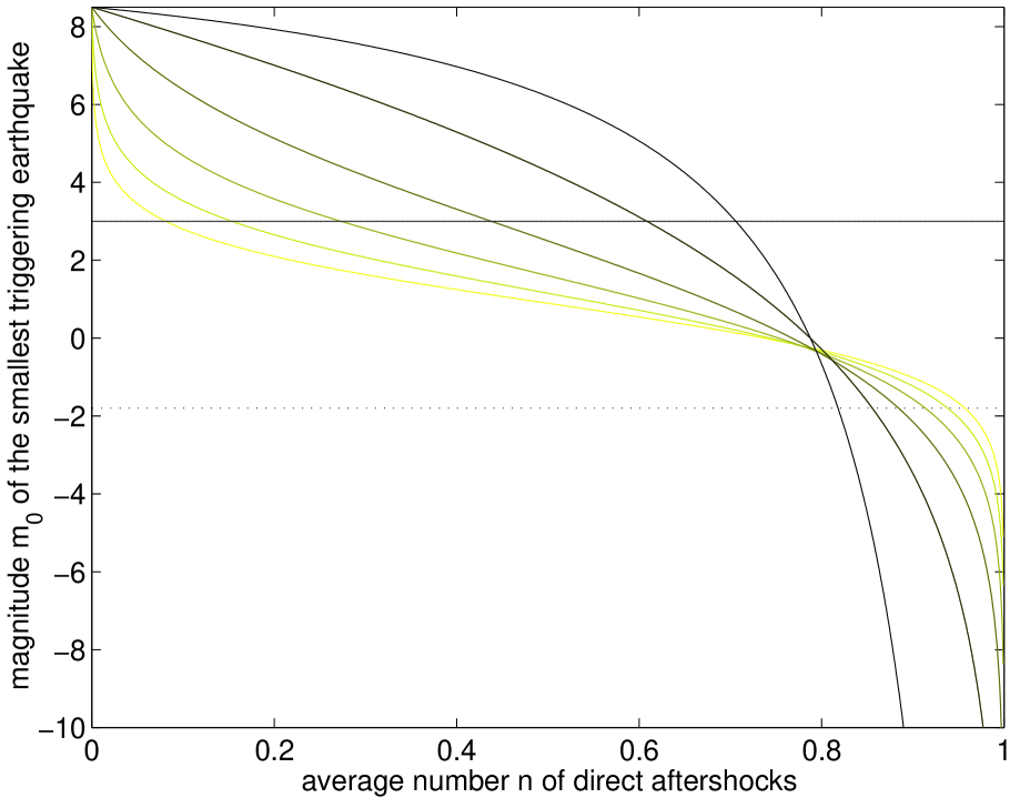
Figure 1: The magnitude $m_{0}$ of the smallest triggering earthquake as a function of the average number $n$ of direct aftershocks estimated from fits to observed aftershock sequences and the ETAS model for values of, from light to dark, $[\alpha=0.5,K_{fit}=0.070]$, $[\alpha=0.6,K_{fit}=0.058]$, $[\alpha=0.7,K_{fit}=0.046]$, $[\alpha=0.8,K_{fit}=0.034]$, $[\alpha=0.9,K_{fit}=0.022]$, $[\alpha=b=1,K_{fit}=0.01]$. Common parameters are $b=1$, $m_{max}=8.5$, $\theta=0.1$, $c=0.001$ days. $K_{fit}$, in units of days^1-p, was estimated by Helmstetter et al. [2004] and herein adapted to these values of $\alpha$ through their correlation (see Figure 2). The horizontal lines represent upper limits of $m_{0}$, derived from the detection threshold $m_{d}=3$ (solid), and from estimates of the critical slip $D_{c}~{}1m$ in rate and state friction giving $m=-1.8$ (dashed), providing conversely a lower bound for the percentage of aftershocks in an earthquake catalog and/or $\alpha$.

The estimate of $m_{0}$ that we are trying to obtain relies on the adequacy of the model used here and on the stability and reliability of the quoted parameters. For now, we sidestep any possible difficulties in the determination of the parameters and present in Figure 1 the magnitude of the smallest triggering earthquake $m_{0}$ as a function of the average number $n$ of direct aftershocks per mainshock for a range of parameters. For $n=0$, $m_{0}$ equals the largest possible earthquake $m_{max}$, representing the limit that earthquakes do not trigger any aftershocks. At the other end, for $n=1$, the formula predicts that $m_{0}$ diverges to minus infinity. Recall that $n=1$ corresponds to the system being exactly at the critical value of a branching process and the statistical average $N_{\rm obs}(m)$ of the total number of events triggered over all generations by a mother event of magnitude $m$ becomes infinite. Of course, individual sequences have a finite lifetime and a finite progeny with probability one and the theoretical average loses its meaning due to the fat-tailed nature of the corresponding distribution [Athreya, 1972; Saichev et al., 2004; Saichev and Sornette, 2004]. Therefore, the prediction on $m_{0}$ becomes unreliable for $n$ close to $1$.

For a wide range of $n$ and combinations between $\alpha$ and $K_{fit}$, the magnitude of the smallest triggering earthquake lies between $0$ and $-10$. Only for values of $n$ above $0.9$ does the size of $m_{0}$ become smaller than $-10$. For reference, a magnitude $-10$ event corresponds to a fault of length $1$mm, i.e. to a typical grain size.

Given that we expect $m_{0}$ to be smaller than the detection threshold $m_{d}$, the horizontal line at $m_{d}=3$ serves as a (very) conservative estimate of the upper limit of $m_{0}$ and thus provides constraints on the combination of parameters $\alpha$, $K_{fit}$ and $n$. For example, for $\alpha=0.5$ and $K_{fit}=0.0702$, at least 10 percent of all earthquakes must be aftershocks. This lower limit increases drastically to about 70 percent for $\alpha=b=1$ and $K_{fit}=0.0095$.

We can obtain another external bound on $m_{0}$ from estimates of the minimum slip required before static friction drops to kinetic friction and unstable sliding begins, according to models of velocity-weakening friction. For example, the parameter $D_{c}$ in rate and state dependent friction [Dieterich, 1992; Dieterich, 1994] was estimated at $0.5$ m from seismograms [Ide and Takeo, 1997] and similarly at $40-90$ cm from slip-velocity records [Mikumo et al., 2003], although both probably correspond to upper bounds. Estimates of $D_{c}$ from laboratory friction experiments are approximately 5 orders of magnitude less than the upper bound determined by seismic studies. One could conclude that either the upper bound from seismic studies is so extreme as to render the comparison to laboratory studies meaningless, or the slip weakening process is in fact different at laboratory scales [Kanamori and Brodsky, 2004]. If we assume that the minimum slip needed to initiate stable sliding corresponds to the minimum length of a friction-based earthquake, then, neglecting fracture-based earthquakes, $D_{c}$ corresponds to the size of the smallest earthquake. Given that the smallest triggering earthquake must be equal to or larger than the smallest earthquake, but that the estimates of $D_{c}$ are upper limits, we use these values for $D_{c}$ as an upper limit of the smallest triggering earthquake. From the relations between fault length, moment and moment magnitude [Kanamori and Brodsky, 2004] with $D_{c}=1$ m and a stress drop of $3$ MPa, we obtain an upper limit of magnitude $-1.8$ for the smallest triggering earthquake. This upper limit is respresented in Figure 1 as the lower horizontal line.

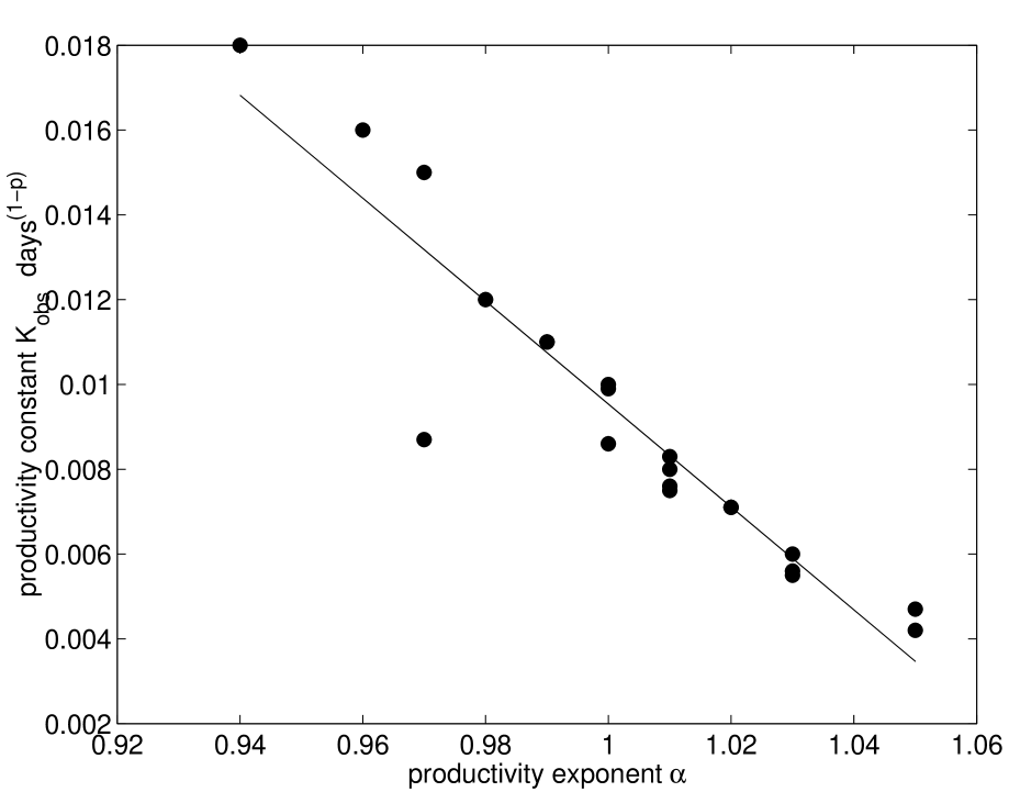
Figure 2: The correlation between the values of $K_{fit}$ and $\alpha$ taken from Table 1 of Helmstetter et al. [2004]. The line is a least-squares fit with slope -0.1214 and y-intercept 0.1309. The extrapolation of this fit for smaller values of $\alpha$ was used to obtain the values for $K_{fit}$ in Figure 1.

Felzer et al. [2002] have used $\alpha=b$ on the basis of an argument of self-similarity. Helmstetter et al. [2004] also argue for a value of $\alpha$ essentially undistinguishable from $b$ based on fits of stacked aftershock decay rates in pre-defined space-time windows. Other studies have found $\alpha$ as small as and even smaller than $0.5$ (see, for example, Console et al. [2003]; Helmstetter [2003]; Zhuang et al. [2004]). In view of the lack of consensus and to keep the discussion independent of the estimation problem, we use the correlation we found between the parameters $K_{fit}$ and $\alpha$ estimated in Helmstetter et al. [2004] to extrapolate to smaller $\alpha$. The existence of such a correlation is standard in joint estimations of several parameters and can be deduced from the inverse of the Fisher matrix of the log-likelihood function Rao [1965]. Such correlation can also be enhanced if the model is misspecified. We performed a least-square fit to the scatter plot (see Figure 2) to obtain a relationship between the parameters and then calculated an estimate of $K_{fit}$ for smaller values of $\alpha$. The resulting curves are plotted in Figure 1.

Delaying the discussion on the estimation problem until the end of the section, we use (12) together with existing estimates of the percentage of aftershocks in seismic catalogs (equivalent to $n$ [Helmstetter and Sornette, 2003b]) to constrain $m_{0}$. We note, however, that different declustering techniques lead to different estimates. No consensus exists on which method should be trusted most. For example, Gardner and Knopoff [1974] found that about 2/3 of the events in the Southern California catalogue are aftershocks. With another method, Reasenberg [1985] found that 48% of the events belong to a seismic cluster. Davis and Frohlich [1991] used the ISC catalog and, out of 47500 earthquakes, found that 30% belong to a cluster, of which 76% are aftershocks and 24% are foreshocks. Recently, using different versions of the ETAS model, Zhuang et al. [2004] have performed a careful inversion of the JMA catalog for Japan using a magnitude $m_{d}=4.2$ for the completeness of their catalog. They provide three estimates of the branching ratio for their best model: $n=0.42$, $0.55$, and $0.46$.

Whether any of these methods estimate $n$ correctly and without bias remains questionable. In particular, the branching ratios as calculated by Zhuang et al. [2004] and others may be significantly biased by the assumption that $m_{d}=m_{0}$, which can be shown to lead to an apparent branching ratio modified by the impact of hidden seismicity below the catalog completeness [Sornette and Werner, 2004]. Moreover, there are problems with the maximum likelihood estimation (see for instance Helmstetter et al. [2004]). However, in the absence of better estimations, we nevertheless use the above values as rough estimates of $n$. Given the range of $\alpha$ and $K_{fit}$, $m_{0}$ is still not very well constrained for one particular value of $n$ (see Figure 1). For example, for 50 percent aftershocks ($n=0.5$), $m_{0}$ ranges from $1$ to an unrealistic $7$ depending on the values of $\alpha$ and $K_{fit}$. This argument could be used to rule out the combination $n=0.5$ and $\alpha=1$. In fact, for $m_{0}$ to be smaller than $m_{d}=3$, at least 70 percent of earthquakes are aftershocks. For $m_{0}$ to be smaller than the upper limit estimated from $D_{c}$, at least 80 percent must be aftershocks.

We can also use the values obtained by Felzer et al. [2003] to constrain $m_{0}$. The authors also used finite space-time windows in which they fitted aftershock sequences with parameters for a global sequence according to

$$C_{T}={A_{T}\over 1-p_{T}}((t+c_{T})^{1-p_{T}}-{c_{T}}^{1-p_{T}}),~{}~{}~{}p_{T}\neq 1,$$ (14)

where $t$ is the selected duration of the sequences, $p_{T}$ is the global Omori exponent, $c_{T}$ is the Omori constant, and $A_{T}$ is the productivity. Assuming that the local Omori exponent is $p=p_{T}=1+\theta_{T}$, expression (14) can be rewritten for the infinite time limit as

$$C_{T}={A_{T}\over\theta_{T}{c_{T}}^{\theta_{T}}}.$$ (15)

The obtained values are listed in Table 3 of their study: $A_{T}=0.116$ days${}^{1-p_{T}}$, $p_{T}=1.08$ and $c_{T}=0.014$ days. These values hold for a typical California aftershock sequence of a magnitude $M_{1}=6.04$ mainshock, a detection threshold of $m_{d}=4.8$, and $\alpha=b=1$.

As before, we equate the ETAS model prediction (8) with the observation (15), eliminate $k$ through expression (6) for $n$ (where $\alpha=b$) and obtain an equation for $m_{0}$ as a function of $n$:

$$m_{0} = m_{max}-{n\over 1-n}{(1-10^{-b(m_{max}-m_{d})})\over b\ln(10)}$$ (16)

$$\times{\theta_{T}c^{\theta_{T}}\over A_{T}}10^{b(M_{1}-m_{d})},~{}~{}~{}~{}~{}\alpha=b=1.$$

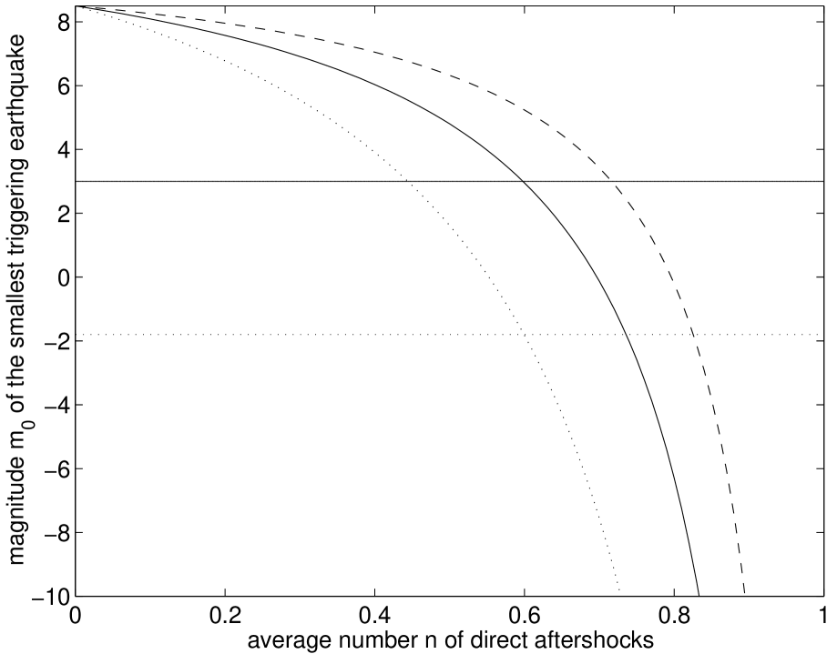
Figure 3: The magnitude $m_{0}$ of the smallest triggering earthquake as a function of the average number $n$ of direct aftershocks estimated from fits to observed aftershock sequences and the ETAS model according to Felzer et al. [2003] (solid), using the parameters $\alpha=b=1$, $m_{max}=8.5$, $\theta_{T}=0.08$, $c_{T}=0.014$ days, $M_{1}=6.04$ and $A_{T}=0.116$ days${}^{1-p_{T}}$. For comparison, we include the curves corresponding to the special case $\alpha=b$ for the fit according to Helmstetter et al. [2004] (dashed) and the constraint due to Båth’s law (dotted) (see 4). The horizontal lines represent upper limits of $m_{0}$, derived from the detection threshold $m_{d}=3$ (solid), and from estimates of the critical slip $D_{c}~{}1m$ in rate and state friction giving $m=-1.8$ (dashed), providing conversely a lower bound for the percentage of aftershocks in an earthquake catalog.

This expression for $m_{0}$ is shown in Figure 3 (solid curve). As in equation (12), $m_{d}$ remains artifactually in the equation due to a dependence of $A_{T}$ on the detection threshold. Since the parameters were obtained with $\alpha=b=1$, we do not alter the values of $\alpha$ and obtain only one curve. For comparison, we include the curve for the case $\alpha=b$ that we obtained above in Figure 1, based on the fits by Helmstetter et al. [2004] (dashed curve) and the curve for the case $\alpha=b$ that results from using Båth’s law (see next section) (dotted). We observe the same characteristics as before in that $m_{0}$ approaches $m_{max}$ for small $n$ and that it diverges to minus infinity for $n$ going to one. Differences between the three curves arise only in the faster or slower decrease of $m_{0}$ with $n$. For example, the (conservative) upper limit $m_{d}=3$ for $m_{0}$ constrains $n$ to be larger than 60 percent according to the values obtained by Felzer et al. [2003], whereas the parameters of Helmstetter et al. [2004] for the case $\alpha=b$ impose $n$ to be at least 70 percent. For the estimate obtained from Båth’s law (see next section), $n$ must be larger than about 45 percent. If we assume that the upper limit of $m_{0}$ can be obtained from estimates of $D_{c}$, corresponding to $m=-1.8$, then $n$ must be at least 60 percent according to the estimate from Båth’s law, 75 percent according to Felzer et al. [2003], and 85 percent according to the fit by Helmstetter et al. [2004]. Conversely, $n=0.7$ determines $m_{0}$ roughly equal to zero, whereas $n=0.8$ implies $m_{0}$ lies in the range $-7$ to $-5$.

Since the three expressions for $m_{0}$ (for $\alpha=b$) show the same functional dependence on key variables and differ only in the different estimates of a few constants, this consistency provides some confidence in our results. As for the difference in the three curves, they constitute three differently formulated, empirical estimates of the number of events of typical aftershock sequences. Given the variability of the aftershock process, the discrepancy in the estimates is to be expected.

We now point out difficulties for exploiting quantitatively the above ideas. Our conclusions for $m_{0}$ and $n$ are based on empirical parameter estimations that involve delicate technical problems. The constants $K_{\rm obs}$ defined in (9) and $A_{T}$ defined in (15) are in principle measurable. Many issues may bias the estimation of these parameters: (i) The total number of aftershocks is estimated empirically in finite space and time windows and events outside are thus missed. In particular, in the special case where $p$, as defined in (2), and $n$ are both close to $1$, a substantial fraction of aftershocks occurs at very long time and are very difficult if not impossible to distinguish from the background seismicity. (ii) Stacking different sequences with different global Omori law decays may introduce errors. (iii) The $p$ exponent of the Omori law may intrinsically depend on the mainshock magnitude [Ouillon and Sornette, 2004]. (iv) Background events may be falsely counted as aftershocks. (v) Magnitude and location uncertainties may bias the parameters. (vi) Missing events in the catalog, especially after large events, may artifactually change the parameter values. (vii) Undetected seismicity may bias the estimated parameters [Sornette and Werner, 2004].

4 Constraints on the smallest triggering earthquake from Bath’s law

Finally, we use the empirical Båth’s law to constrain $m_{0}$ as a function of $n$. The law states that the average difference between a mainshock of magnitude $M_{1}$ and the magnitude $m_{a}$ of its largest aftershock is $dm=M_{1}-m_{a}=1.2$, regardless of the mainshock magnitude (see for example Helmstetter and Sornette, [2003a] and references therein). Let $N_{obs}$ be the total number of aftershocks generated by the mainshock above the magnitude $m_{d}$ of completeness of the catalog. Assuming that the magnitudes of the aftershocks are drawn from the Gutenberg-Richter law, the largest aftershock has an average magnitude given by a simple argument of extreme value theory:

$$m_{a}=m_{d}+(1/b)(\log_{10}N_{obs})~{}.$$ (17)

Solving this expression for $N_{obs}$, equating it with the ETAS prediction (8) and eliminating $k$ through the expression for $n$ (6) provides an estimate of $m_{0}$ as a function of $n$:

$$m_{0}={1\over(\alpha-b)\ln(10)}\times$$

$$\ln 10^{(\alpha-b)m_{max}}+{b-\alpha\over b}{n\over 1-n}~{}10^{\alpha M_{1}-bm_{a}}~{}(1-10^{-b(m_{max}-m_{d})}),$$ (18)

for $\alpha\neq b$ and

$$m_{0}=m_{max}-({n\over 1-n}){(1-10^{-b(m_{max}-m_{d})})\over b\ln(10)}~{}10^{b(M_{1}-m_{a})}~{},$$ (19)

for $\alpha=b$.

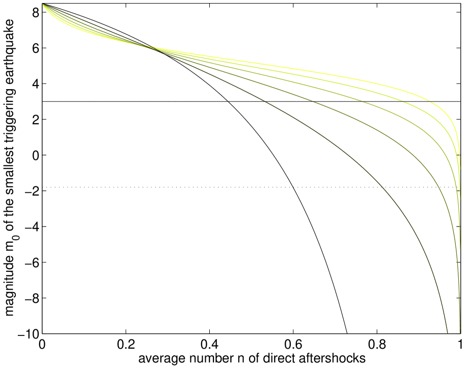
Figure 4: The magnitude $m_{0}$ of the smallest triggering earthquake as a function of the average number $n$ of direct aftershocks as estimated by the ETAS model and Båth’s law for $\alpha=[0.5,0.6,0.7,0.8,0.9,1]$, from light to dark. The horizontal lines represent upper limits of $m_{0}$, derived from the detection threshold $m_{d}=3$ (solid), and from estimates of the critical slip $D_{c}~{}1m$ in rate and state friction giving $m=-1.8$ (dashed), providing conversely a lower bound for the fraction $n$ of aftershocks in an earthquake catalog and/or $\alpha$. Common parameters are $b=1$, $m_{max}=8.5$, $m_{main}=7$, $m_{a}=5.8$.

Figure 4 illustrates the behaviour of $m_{0}$ as a function of the average number $n$ of direct aftershocks for reasonable values of the other constants ($m_{max}=8.5$, $m_{d}=3$, $b=1$, $\alpha=[0.5,0.6,0.7,0.8,0.9,1]$ (light to dark)), for mainshock and largest aftershock values according to $M_{1}-m_{a}=7-5.8=1.2$ from Båth’s law. Again, as $n$ tends to one, $m_{0}$ tends to minus infinity, while for $n=0$, $m_{0}=m_{max}$, as expected. We also observe that $m_{0}$ is almost constant over a wide range of $n$ for comparatively small $\alpha$, whereas $m_{0}$ varies much faster for the case $\alpha=b$.

As alluded to in the last section, we obtain the same functional dependence as in both previous estimates of the last section. However, for $\alpha=b$, the decrease of $m_{0}$ with increasing $n$ is even faster than when using the parameters of Felzer et al. [2003]. Here, the upper limit $m_{d}=3$ for $m_{0}$ (upper horizontal line) constrains $n$ to be larger than 45 percent, smaller than the 60 percent found previously. This discrepancy is due to the three different ways of estimating the observed number of aftershocks. However, since all three are in a similar range, they provide a test of the consistency of the results.

When applying the $D_{c}$-derived upper limit of $-1.8$ (lower horizontal line), $n$ must be larger than at least 60 percent for $\alpha=b$ and larger than 80 percent for $\alpha=0.9$. We thus find that for $n=0.5$, $m_{0}$ is in the range $2$ to an unrealistic $5$, while for $n=0.7$, $m_{0}$ lies between $-10$ and $5$, depending on the values of $\alpha$. Since $m_{0}\geq 3$ is unrealistic, the entire region of combinations between $\alpha$ and $n$ that fall above that value can be ruled out. For example, the case $\alpha=0.8$ leads to a reasonable $m_{0}$ smaller than $m_{d}=3$ only for $n$ larger than about 65 percent.

5 Conclusions

We have shown that differentiating between the smallest triggering earthquake $m_{0}$ and the detection threshold $m_{d}$ within the ETAS model leads, together with three separate estimates of the observed numbers of aftershocks, to three estimates of $m_{0}$ as a function of the percentage $n$ of aftershocks in a catalog (also equal to the branching ratio). We have used empirically fitted values for aftershock numbers and thereby eliminated one variable from the ETAS formalism in order to obtain an estimate of $m_{0}$ as a function of $n$. The three different estimates were obtained from the fits performed by Helmstetter et al. [2004], by Felzer et al. [2003], and from the empirical Båth’s law (see Helmstetter and Sornette [2003a] and references therein). All three give the same functional dependence and similar values for $m_{0}$. In particular, we can place bounds on $m_{0}$ from estimates of the percentage of aftershocks in earthquake catalogs. Conversely, we can limit the range of $n$ by observing that $m_{0}$ must be less than the detection threshold $m_{d}$, or, less conservatively, that $m_{0}$ must be less than the magnitude corresponding to the rate-and-state critical slip $D_{c}$ as estimated from seismograms. Apart from quantitative values for $m_{0}$, the bounds limit the possible combinations between $n$ and $\alpha$ and, in particular, indicates that at least 60 to 70 percent of all earthquakes are aftershocks.

The fact that the existence of a small magnitude cut-off $m_{0}$ for triggering should have observable consequences may appear surprising. But such a phenomenon of the impact of a small scale cut-off on “macroscopic” observables is not new in physics and actually permeates particle physics, field theory and condensed matter physics. In the present case, the existence of $m_{0}$ has an observable impact especially when $\alpha\leq b$ for which the cumulative effect of tiny earthquakes dominate or equate that of large earthquakes with respect to the physics of triggering other earthquakes [ Helmstetter, 2003; Helmstetter et al., 2004]. We hope that the present article, together with our companion paper Sornette and Werner [2004], will draw the attention of the community to the important problem of the distinction between $m_{d}$ and $m_{0}$. Moreover, it will perhaps encourages re-analyses of inversion methods of models of triggered seismicity, and in particular of maximum likelihood estimations, to take into account the bias due to the unobserved seismicity below the magnitude of catalog completeness.