eurm10 \checkfontmsam10 \blacksquare
Part I X
XXX
Modulated dust-acoustic wave packets
in a plasma with non-isothermal
electrons and ions
Abstract
Nonlinear self-modulation of the dust acoustic waves is studied, in the presence of non-thermal (non-Maxwellian) ion and electron populations. By employing a multiple scale technique, a nonlinear Schrödinger-type equation (NLSE) is derived for the wave amplitude. The influence of non-thermality, in addition to obliqueness (between the propagation and modulation directions), on the conditions for modulational instability to occur is discussed. Different types of localized solutions (envelope excitations) which may possibly occur are discussed, and the dependence of their characteristics on physical parameters is traced. The ion deviation from a Maxwellian distribution comes out to be more important than the electron analogous deviation alone. Both yield a de-stabilizing effect on (the amplitude of) DAWs propagating in a dusty plasma with negative dust grains, and thus favor the formation of bright- (rather than dark-) type envelope structures (solitons) in the plasma. A similar tendency towards amplitude de-stabilization is found for the case of positively charged dust presence in the plasma.
1 Introduction
Dust contaminated plasmas have recently received considerable interest due to their wide occurrence in real charged particle systems, both in space and laboratory plasmas, and to the novel physics involved in their description [[1, 2]]. An issue of particular interest is the existence of special acoustic-like oscillatory modes, e.g. the dust-acoustic wave (DAW) and dust-ion-acoustic wave (DIAW), which were theoretically predicted about a decade ago [[3, 4]] and later experimentally confirmed [[5, 6]]. The DAW, which we consider herein, is a fundamental electrostatic mode in an unmagnetized dusty plasma (DP), which has no analogue in an ordinary e-i (electron - ion) plasma. It represents electrostatic oscillations of mesoscopic size, massive, charged dust grains against a background of electrons and ions which, given the low frequency of interest, are practically in a thermalized (i.e. Boltzmann) equilibrium state. The phase speed of the DAW is much smaller than the electron and ion thermal speeds, and the DAW frequency is below the dust plasma frequency.
The amplitude (self-) modulation of the DAse waves has been recently considered [[7] - [9]], by means of the reductive perturbation formalism [[10]]. A study of the modulational stability profile of DA waves has shown that long/short wavelength DA waves are stable/unstable against external perturbations. The respective parameter regions are associated with the occurrence of localized envelope excitations of the dark/bright type (i.e. voids/pulses). Obliqueness in perturbations are found shown to modify this dynamic behaviour [[7] - [9]].
Allowing for a departure from Boltzmann’s distribution for the electrostatic background (non-thermality) has been shown to bear a considerable effect on electrostatic plasma modes. Inspired by earlier works on the ion-acoustic (IA) solitary waves [[11]], recent studies have shown that the presence of a non-thermal ion velocity distribution may modify the nonlinear behaviour of the DA waves, affecting both the form and the conditions for the occurrence of the DA solitons [[12, 13]]. Also, the self-modulation of IA waves was recently shown to be affected by the electron non-thermality [[14]]. However, no study has been carried out of the effect of a non-thermal ion and/or electron background population on the modulation properties of the DA waves. This paper aims at filling this gap.
2 The model
Let us consider the propagation of the dust-acoustic waves in an unmagnetized dusty plasma. The mass and charge of dust grains (both assumed constant, for simplicity) will be denoted by and , where denotes the sign of the dust charge (). Similarly, we have: and for ions, and and for electrons. The typical DAW frequency will be assumed much lower than the (inverse of the) characteristic dust grain charging time scale, so charge variation effects (known to lead to collisionless wave damping) will be omitted here.
The basis of our study includes the moment - Poisson system of equations for the dust particles and non-Boltzmann distributed electrons and ions. The dust number density is governed by the continuity equation
| (1) |
and the dust mean velocity obeys
| (2) |
where is the electric potential. The dust pressure dynamics (i.e. the dust temperature effect) is omitted within the cold dust fluid description. The system is closed by Poisson’s equation
| (3) |
Overall neutrality, viz.
is assumed at equilibrium.
2.1 Non-thermal background distribution(s)
Following the model of Cairns et al. [[11]], the non-thermal velocity distribution for (electrons) and (ions) is taken to be
| (4) |
where , and denote the equilibrium density, temperature and thermal speed of the species , respectively. The real parameter expresses the deviation from the Maxwellian state (which is recovered for ). Integrating over velocities, Eq. (4) leads to
| (5) |
[[11]], where and ; the normalized potential variables are , where is the ion/electron charge state.
2.2 Reduced model equations - weakly nonlinear oscillations
The above system of evolution equations for the dust fluid can be cast into the reduced (dimensionless) form:
| (6) |
and
| (7) |
where the particle density , mean fluid velocity , and electric potential are scaled as: , , and , where is the equilibrium dust density; the effective temperature is related to the characteristic dust speed , defined below ( is Boltzmann’s constant). Time and space variables are scaled over the characteristic dust period (inverse dust plasma frequency) , and the effective Debye length, defined as [where is the Debye length for species ; the non-thermality parameters are defined below]. The (unperturbed) dust Debye length is also defined.
Near equilibrium (), Poisson’s Eq. (3) becomes:
| (8) |
Note that the right-hand side in Eq. (8) cancels at equilibrium. Here,
and
For , one may retain the approximate expressions: and ; also, in this case (notice that the dependence on the electron parameters disappears in this approximation). We have defined the dust parameter ; see that is lower (higher) than unity for negative (positive) dust charge, i.e. for ().
The dust parameter , together with the temperature ratio , are the (dimensionless) physical parameters essentially affecting our problem. For instance, see that (defined above) may be expressed as: .
3 Perturbative analysis
Following the reductive perturbation technique [[10]], we define the state vector , whose evolution is governed by Eqs. (6) - (8), and then expand all of its elements in the vicinity of the equilibrium state , viz. , where is a smallness parameter. We assume that (for ; we impose , for reality), thus allowing the wave amplitude to depend on the stretched (slow) coordinates and , where () (bearing dimensions of velocity) will be determined later. Note that the choice of direction of the propagation remains arbitrary, yet modulation is allowed to take place in an oblique direction, characterized by a pitch angle . Having assumed the modulation direction to define the axis, the wave vector is taken to be .
According to the above considerations, the derivative operators in the above equations are treated as
and
i.e. explicitly
and
for any of the components of .
3.1 First harmonic amplitudes
Iterating the standard perturbation scheme [[10]], we obtain the first harmonic amplitudes (to order )
| (9) |
which may be expressed in terms of a sole state variable, e.g. the potential correction . The well-known DA wave (reduced) dispersion relation is also obtained, as a compatibility condition.
The amplitudes of the 2nd and 0th (constant) harmonic corrections are obtained in order (the lengthy expressions are omitted for brevity). Furthermore, the condition for suppression of the secular terms leads to the compatibility condition: ; therefore, bears the physical meaning of a group velocity in the direction of amplitude modulation ().
3.2 The envelope evolution equation
The potential correction obeys an explicit compatibility condition in the form of the nonlinear Schrödinger–type equation (NLSE)
| (10) |
The dispersion coefficient is related to the curvature of the dispersion curve as ; the exact form of P reads
| (11) |
The nonlinearity coefficient , due to carrier wave self-interaction, is given by a complex function of , and . Distinguishing different contributions, can be split into three distinct parts, viz.
| (12) |
where
| (13) | |||||
| (14) | |||||
| (15) | |||||
One may readily check, yet after a tedious calculation, that expressions (13) and (15) reduce to (53) and (54) in Ref. [7] (for a Maxwellian distribution, i.e. setting in all formulae above); notice however, that the term was absent therein. Note that only (which is related to self-interactions due to the zeroth harmonic) depends on the angle (and is, in fact, an even, periodic function of ).
4 Stability profile – envelope excitations
The evolution of a wave whose amplitude obeys Eq. (10) essentially depends on the sign of the product (see, e.g., in Ref. [16] for details; also see in Refs. [9] and [17]) which may be numerically investigated in terms of the physical parameters involved.
For , the DA wave is modulationally unstable and may either collapse, when subject to external perturbations, or evolve into a series of bright-type localized envelope wavepackets, which represent a pulse-shaped solution of the NLSE (10). This type of solution is depicted in Fig. 2.
For , on the other hand, the DA wave is stable and may propagate as a dark/grey-type envelope wavepacket, i.e. a propagating localized envelope hole (a void) amidst a uniform wave energy region. Notice the qualitative difference between the dark and grey solutions (depicted in Fig. 3a and b, respectively): the potential vanishes in the former, while it remains finite in the latter.
The exact analytical expressions for different types of envelope excitations (depicted in Figs. 2 and 3) are summarized in Refs. [9] and [17]; more details can be found in Ref. [18]. We note that, in either case (i.e. for positive or negative product ), the localized excitation width and maximum amplitude satisfy . The dynamics, therefore, essentially depends on the quantity , whose sign (magnitude) will determine the wave’s stability profile and the type (characteristics, respectively) of the localized envelope excitations which may occur.
5 Numerical analysis
According to the above analysis, both the DAW stability profile and the type of DA envelope excitations possibly occurring in the plasma are determined by the sign of the product of the NLSE coefficients and , which is essentially a function of the wavenumber (normalized by [[19]]), the dust parameter , the temperature ratio and the non-thermality parameters , in addition to the modulation angle . The exact expressions obtained for and may now be used for the numerical investigation of the wave’s modulational stability profile.
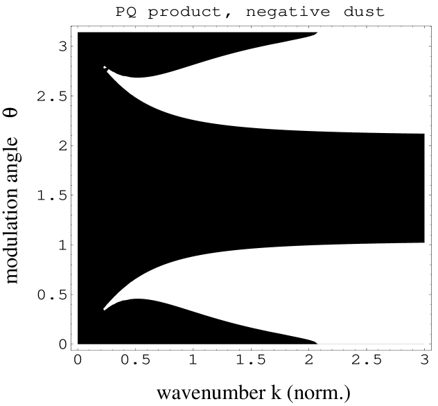
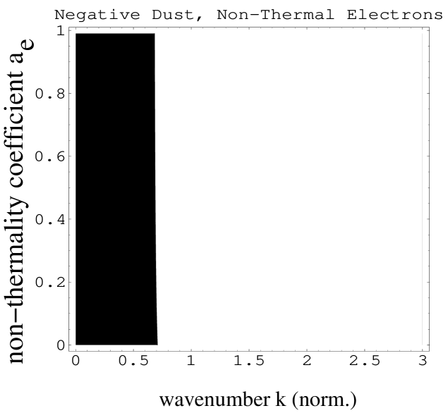
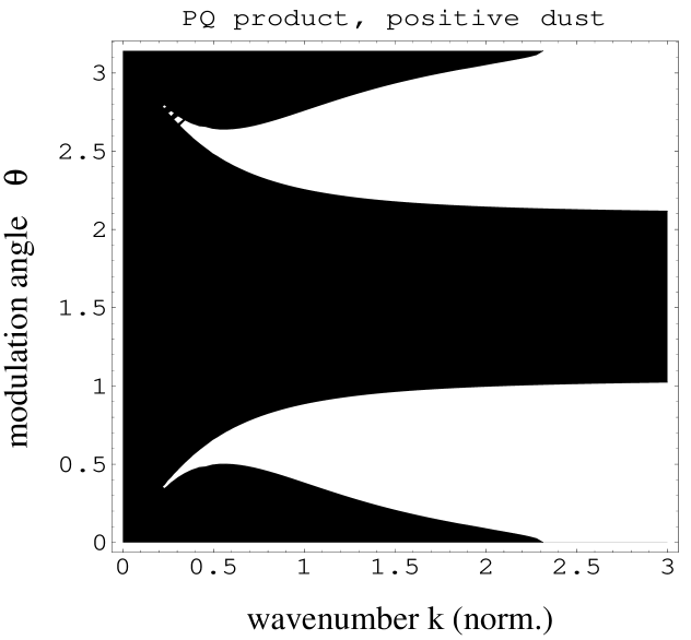
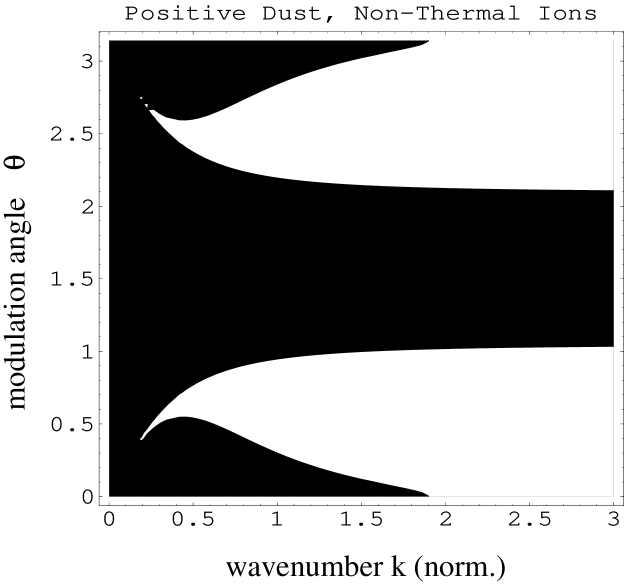
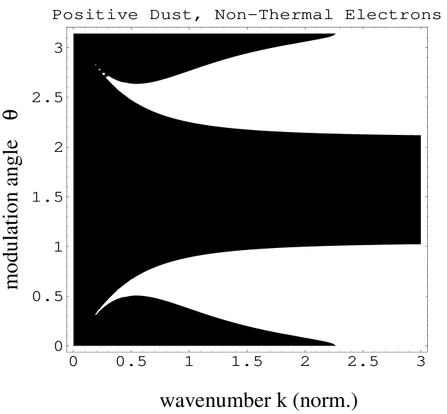
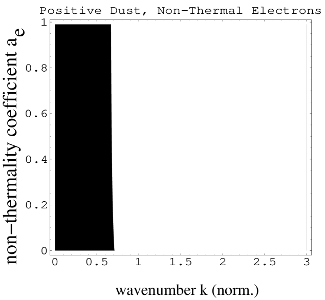
In the figures provided here (see Figs. 4 - 9), the black/white regions represent a negative/positive sign, implying DAW being modulationally stable/ unstable (and possibly propagating in the form of dark/bright type excitations, respectively).
Throughout this Section, we have used the set of representative values: , and , implying for negatively charged dust (and for positively dust charge; cf. the definitions above). The (normalized) wavenumber , modulation angle () and the non-thermality parameters () will be allowed to vary according to the focus of our investigation. The negative dust charge case () is implied, unless otherwise mentioned.
5.1 Parallel modulation
In the special case of the parallel modulation (), the analytical behaviour of and was briefly studied in Ref. [15]. See that for so that one only has to study the sign of . For one then obtains the approximate expression [[15]]: and , which prescribes stability (and dark/grey type envelope excitations – voids) for long wavelengths. For shorter wavelengths, i.e. for (where is some critical wavenumber, to be determined numerically), changes sign (becomes negative), and the wave may become unstable.
In addition to the above results, an increase in the non-thermal ion population (i.e. in the value of ) is seen to favor instability at lower values of : see that the black region shrinks - for - when passing from Fig. 4a to Fig. 4b. Large wavelengths always remain stable and may only propagate as dark-type excitations. On the other hand, the effect of an increase in the non-thermal electron population (i.e. in the value of ), while keeping ions Maxwellian, has a similiar, yet not so dramatic effect; cf. Fig. 4c, for . We note that the effect of non-thermality (of ions, in particular) on the parallel modulation of a dusty plasma with positively charged dust is qualitatively similar; compare e.g. Fig. 4b to Fig. 7b (for ).
5.2 Obliqueness effects
Let us now consider an arbitrary value of . First, we note that, for small wavenumber , one obtains: and , so that stability (and the existence of dark/grey type excitations) is, again, ensured for long wavelengths .
We proceed by a numerical investigation of the sign of the coefficient product in the plane; see Fig. 4. The profile thus obtained is qualitatively reminiscent of the results in Ref. [9]: the critical wavenumber, say , beyond which changes sign, decreases as the modulation obliqueness angle increases from zero (parralel modulation) to - roughly - 0.5 rad (i.e. approximately ), implying a destabilization of the DAW amplitude for lower wave number (higher wavelength) values. Now, above 0.5 rad (i.e. ), approximately, and up to rad (i.e. , transverse modulation) the wave remains stable.
A question naturally arises at this stage: how does the forementioned stability profile depend on the non thermal character of the background? The ion and electron non-thermality effects are separately treated in the following paragraphs.
5.3 Ion non-thermality effects
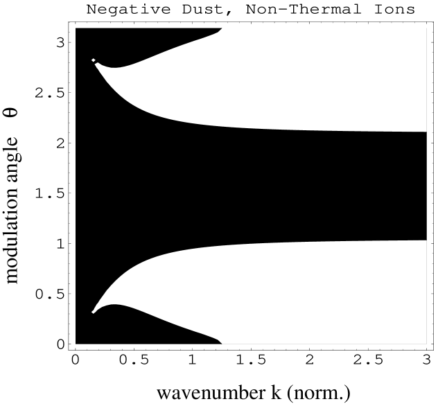
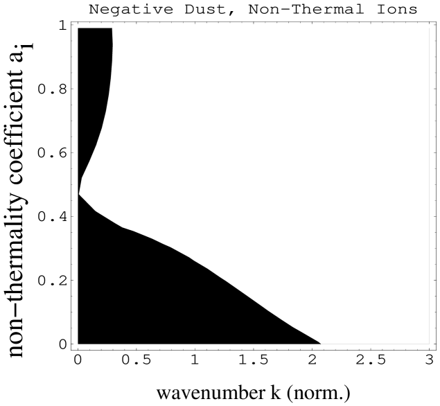
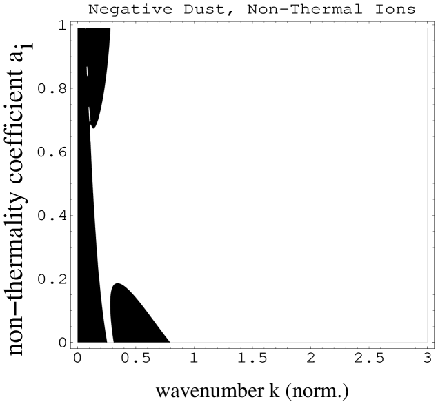
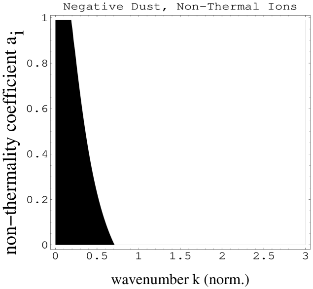
Let us vary the value of the ion non-thermality parameter . Passing to a finite value of results in a narrower stability region for small angles (i.e. , at which , decreases with , for small ) – see Fig. 4b – while the influence on the behaviour for larger angles is less important. Therefore, a small non Maxwellian ion population (for less than 0.2, roughly) seems to slightly enhance modulational instability (i.e. destroy stability) at lower wavenumber values, at least for a small to moderate modulation obliqueness. Slightly higher values of rather favor instability even further. Finally, the picture is reversed for very high (above, say, 0.5), where the wave is slightly stabilized by increasing (at least for moderate values of ). These effects may be depicted by keeping the value of fixed, while varying the value of ; see Figs. 5. The influence of non-thermality on strongly oblique DAW modulation is tacitly negative: stability is destroyed by increasing (see e.g. Fig. 5c, where ). The transverse DAW modulation case (i.e. for ) remains globally stable, so the corresponding (black) diagram was omitted in Fig. 5.
5.4 Electron non-thermality effects
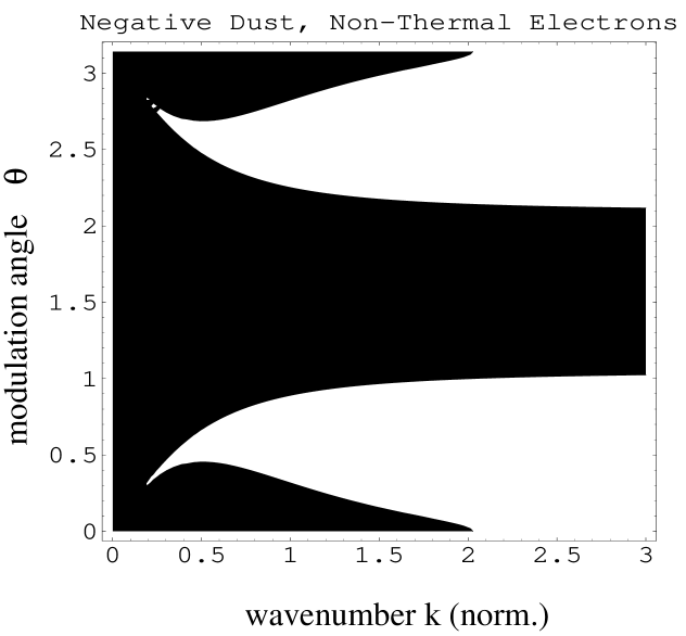
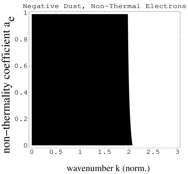
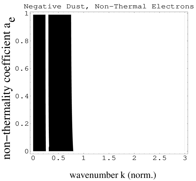
In analogy to the previous paragraph, we may now vary the value of the electron non-thermality parameter . The effect is qualitatively similar, yet far less dramatic; see Fig. 6. This is physically expected, since the influence of the background ions on the inertial dust grains is more important than that of the lighter electrons.
5.5 Positive dust
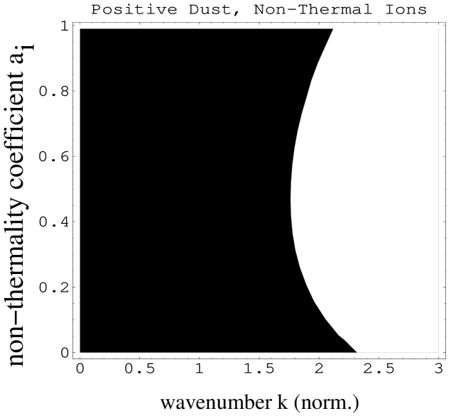
The analogous investigation in the positive dust case (; everywhere below) reveals a qualitatively different picture. Again, the addition of positive dust is seen to result in a much narrower stability region; compare Figs. 4 and 7. We see that positive dust slightly favors instability, with respect to negative dust; cf. the discussion in Ref. [9].
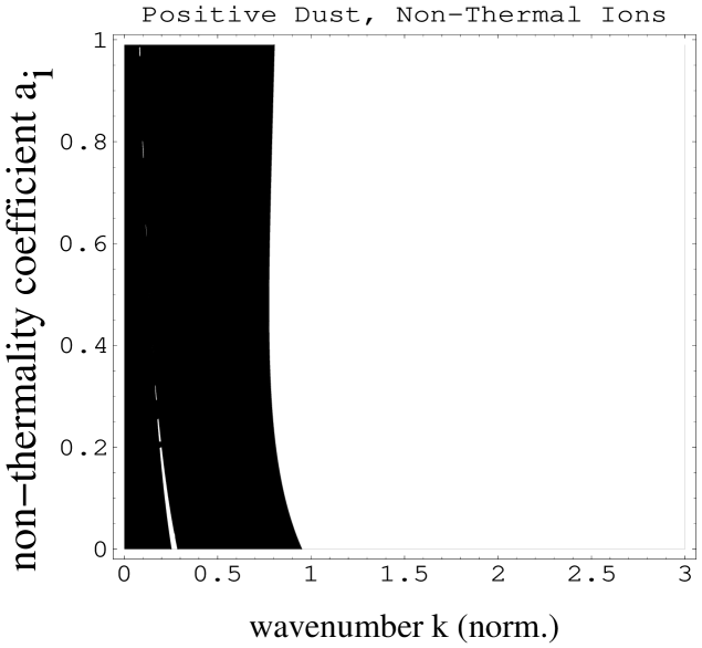
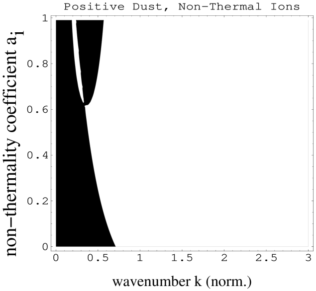
As far as the influence of ion non-thermality on stability is concerned, the qualitative effect seems to be the opposite as in the preceding paragraphs. For a given value of the angle , increasing the ion “non-Maxwellian” parameter seems to result in a more unstable configuration, i.e. in a narrower black region in Fig. 8, for ; this is true for values of up to, say, 0.5, while reaching higher ones bears the opposite effect (see the upper half of Fig. 8a). For higher , the result is similar, yet less dramatic; see Figs 8b, c. Again (as in the positive dust charge case), the transverse DAW modulation case (i.e. for ) remains globally stable, so the corresponding (completely black) diagram was omitted in Fig. 8.
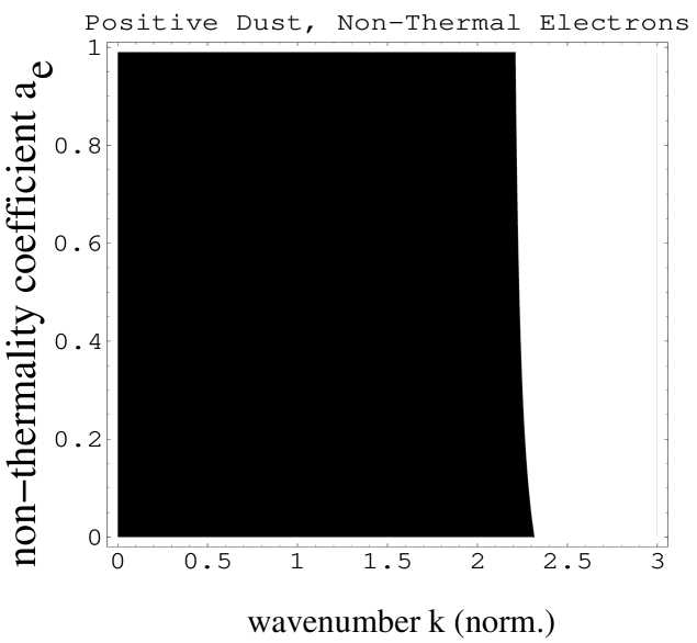
Finally, taking into account electron non-thermality, i.e. increasing the electron parameter from zero to a finite value yields a similar effect, yet much less important effect, for practically all values of and .
In conclusion, the modulational instability of DAWs propagating in a dusty plasma with positively charged dust grains seems to be enhanced by the appearance of a non-thermal background component.
6 Conclusions
We have investigated the amplitude modulation of dust acoustic waves in the presence of a non-thermal (non-Maxwellian) ion and/or electron background, focusing on the influence of the latter on the stability profile, and also on the conditions for the occurrence of envelope excitations.
Summarizing our results, we find that the presence of non-Maxwellian electron an/or ion distribution(s) is expected to yield a destabilizing effect on the DAW propagation in a plasma with negatively charged dust grains (slightly favoring dark- rather than bright-type envelope wave packets), in particular for a moderate obliqueness in amplitude perturbation. This effect is (qualitatively similar but) stronger for nonthermal ions rather than electrons. In the presence of a transverse modulation, the wave’s stability profile remains intact. The modulational instability of the DAWs propagating in a dusty plasma with positively charged dust grains () also seems to be enhanced by the appearance of a nonthermal electron and ion components. Again, this effect is stronger for nonthermal ions rather than electrons; also, transversely modulated DAWs remain stable.
Finally, the occurrence of bright (rather than dark) type envelope wave packets is rather favored by deviations of the ion (and electron, though less) population(s) from the Maxwellian distribution.
Therefore, adding a non thermal ion and/or electron component to the plasma may control (and possibly stabilize) the propagation of dust-acoustic envelope solitons, by enhancing energy localization via instability of the wave’s amplitude (due to carrier self-modulation).
Acknowledgements.
This work was supported by the DFG (Deutscheforschungsgemeischaft) through the Programme SFB591 (Sonderforschungsbereich) – Universelles Verhalten gleichgewichtsferner Plasmen: Heizung, Transport und Strukturbildung. The authors are happy to dedicate this article to Robert Alan Cairns on the occasion of his 60th birthday.19
References
- [1] Verheest, F. 2001 Waves in Dusty Space Plasmas, Kluwer Academic Publishers, Dordrecht.
- [2] Shukla, P. K. & Mamun, A. A. 2002 Introduction to Dusty Plasma Physics, Institute of Physics Publishing Ltd., Bristol.
- [3] Rao, N. N., Shukla, P. K. & Yu, M. Y. 1990 Dust-acoustic waves in dusty plasmas Planet. Space Sci. 38, 543–546.
- [4] Shukla, P. K. & Silin, V. P. 1992 Dust-ion acoustic wave Phys. Scr. 45, 508.
- [5] Barkan, A. Merlino, R. & D’Angelo, N. 1995 Laboratory observation of the dust acoustic wave mode Phys. Plasmas 2 (10), 3563 – 3565.
- [6] Pieper, J. & Goree, J. 1996 Dispersion of Plasma Dust Acoustic Waves in the Strong Coupling Regime Phys. Rev. Lett. 77, 3137 – 3140.
- [7] Amin, M. R., Morfill, G. E. and Shukla, P. K., 1998 Amplitude Modulation of Dust-Lattice Waves in a Plasma Crystal Phys. Rev. E 58, 6517 – 6523.
- [8] Tang, R. & Xue, J. 2003 Stability of oblique modulation of dust-acoustic waves in a warm dusty plasma with dust variation Phys. Plasmas 10, 3800 – 3803.
- [9] Kourakis, I. & Shukla, P. K. 2004 Oblique amplitude modulation of dust-acoustic plasma waves Phys. Scripta 69 (4), 316 – 327.
- [10] Taniuti, T. & Yajima, N. 1969 Perturbation method for a nonlinear wave modulation J. Math. Phys. 10, 1369 – 1372; Asano, N. Taniuti, T. & Yajima, N. 1969 Perturbation method for a nonlinear wave modulation II J. Math. Phys. 10, 2020 – 2024.
- [11] Cairns, R. A. et al. 1995 Electrostatic solitary structures in non-thermal plasmas Geophys. Res. Lett. 22, 2709 – 2712.
- [12] Gill, T, S. & Kaur, H. 2000 Effect of nonthermal ion distribution and dust temperature on nonlinear dust acoustic solitary waves Pramana J. Phys. 55 (5 & 6), 855 – 859.
- [13] Singh, S.V., Lakhina, G. S., Bharuthram R. and Pillay S. R. 2002 Dust-acoustic waves with a non-thermal ion velocity distribution, in Dusty plasmas in the new Millenium, AIP Conf. Proc. 649 (1), 442 – 445.
- [14] Xue, J. 2003 Modulational instability of ion-acoustic waves in a plasma consisting of warm ions and non-thermal electrons Chaos, Solitons and Fractals 18, 849 – 853; Tang, R. & Xue, J. 2004 Non-thermal electrons and warm ions effects on oblique modulation of ion-acoustic waves Phys. Plasmas 11 (8), 3939 – 3944.
- [15] Kourakis, I. & Shukla, P. K. 2004 Modulational instability and envelope excitations of dust-acoustic waves in a non–thermal background Proc. 31st EPS Plasma Phys. (London, UK), European Conference Abstracts (ECA) Vol. 28B, P-4.081, Petit Lancy, Switzerland).
- [16] Hasegawa, A. 1975 Plasma Instabilities and Nonlinear Effects, Springer-Verlag, Berlin.
- [17] Kourakis, I. & Shukla, P. K. 2004 Nonlinear Modulated Envelope Electrostatic Wavepacket Propagation in Plasmas Proc. 22nd Sum. Sch. Int. Symp. Phys. Ionized Gases (SPIG 2004, Serbia and Montenegro), AIP Proceedings Series, USA (to appear).
- [18] Fedele, R., Schamel, H. and Shukla, P. K. 2002 Solitons in the Madelung’s Fluid Phys. Scripta T98 18 – 23; also, Fedele, R. and Schamel, H. 2002 Solitary waves in the Madelung’s Fluid: A Connection between the nonlinear Schrödinger equation and the Korteweg-de Vries equation Eur. Phys. J. B 27 313 – 320.
-
[19]
For rigor, the (reduced) parameter (i.e. essentially
, where is the wavelength)
appearing in the formulae,
has had to be redefined as , in order to be
represented in the horizontal axis in Figs. 4 - 9
(where the normalized variable is now ).
Figure captions
Figure 1: The non-thermal distribution , as defined by Eq. (4) [scaled by ], vs. the reduced velocity , for 0, 0.1, 0.2, 0.3 (from top to bottom).
Figure 2: Bright type localized envelope modulated wavepackets (for ) for two different (arbitrary) sets of parameter values.
Figure 3: (a) Dark and (b) grey type localized envelope modulated wavepackets (for ). See that the amplitude never reaches zero in the latter case.
Figure 4: The sign of the product is depicted vs. (normalized) wavenumber (horizontal axis) and modulation angle (vertical axis), via a color code: black (white) regions denote a negative (positive) sign of , implying stability (instability), and suggesting dark (bright) type envelope soliton occurrence. Here, (negative dust charge) and: (a) (Maxwellian background); (b) , (ion non-thermality); (c) , (electron non-thermality). Remaining parameter values as cited in the text. See that the effect in (c) is rather negligible.
Figure 5: The sign of the product is depicted vs. (normalized) wavenumber (horizontal axis) and ion non-thermality parameter (vertical axis), for a modulation angle equal to: (a) 0 (parallel modulation); (b) 0.4; (c) ; the case – transverse modulation – is omitted, since globally stable. Same color code as in Fig. 4: black (white) regions denote a negative (positive) sign of . Here, (negative dust charge) and (Maxwellian electrons). Remaining parameter values as cited in the text.
Figure 6: Similar to the preceding Figure, but for non-thermal electrons and Maxwellian ions: the sign of the product is depicted vs. (normalized) wavenumber (horizontal axis) and electron non-thermality parameter (vertical axis), for a modulation angle equal to: (a) 0 (parallel modulation); (b) 0.4; (c) ; the case – transverse modulation – is omitted, since globally stable. Same color code as in Fig. 4: black (white) regions denote a negative (positive) sign of . Here, (negative dust charge) and (Maxwellian ions). Remaining parameter values are cited in the text.
Figure 7: Similar to Figure 4, but for a positive dust charge; here, . The sign of the product is depicted vs. (normalized) wavenumber (horizontal axis) and modulation angle (vertical axis), for: (b) , (ion non-thermality); (c) , (electron non-thermality). Remaining parameter values as in Fig. 4. See that the effect in (c) is not as dramatic as in (b).
Figure 8: Similar to Figure 5, but for a positive dust charge; here, and (remaining parameter values as in Fig. 5). The sign of the product is depicted vs. (normalized) wavenumber (horizontal axis) and ion non-thermality parameter (vertical axis), for a modulation angle equal to: (a) 0 (parallel modulation); (b) 0.4; (c) ; the case – transverse modulation – is omitted, since globally stable.
Figure 9: Similar to Figure 6, but for a positive dust charge; here, and (remaining parameter values as in Fig. 6). The sign of the product is depicted vs. (normalized) wavenumber (horizontal axis) and electron non-thermality parameter (vertical axis), for a modulation angle equal to: (a) 0 (parallel modulation); (b) 0.4; (c) ; the case – transverse modulation – is omitted, since globally stable. See that the electron non-thermality effect is less important than its ion counterpart (cf. Fig. 6).


(a)

(b)

(a)

(b)
(a)
(b)
(c)
(a)
(b)
(c)
(a)
(b)
(c)
(a)
(b)
(c)
(a)
(b)
(c)
(a)

(b)
(c)