On a possible dynamical scenario leading to a generalised Gamma distribution

Abstract

In this report I present a possible scenario which can lead to the emergence of a generalised Gamma distribution first presented by C Tsallis et al. as the distribution of traded volumes of stocks in financial markets. This propose is related with superstatics and the notion of moving average commonly used in econometrics.

I The $\Gamma$-distribution

The $\Gamma$-distribution is a general distribution that is verified in processes where the waiting times between variables that follow a Poisson distribution are significant. It involves two free parameters, usually labeled by $\alpha$ and $\theta$ and defined as [1],

$$p_{\alpha,\theta}\left(x\right)=\frac{x^{\alpha-1}\exp\left(-\frac{x}{\theta}\right)}{\Gamma\left[\alpha\right]\,\theta^{\alpha}}.$$ (1)

A special case of $\Gamma$-distribution is to consider $\alpha=r/2$ and $\theta=2$. In this case the distribution is called $\chi^{2}$-distribution and represents the probability of get a value $\zeta$ of a variable that is obtained by the summation of $r$ independent squared variables $\xi_{i}$ associated with the Gaussian distribution with null mean and unitary variance [1],

$$\zeta=\sum\limits_{i=1}^{r}\xi_{i}^{2}.$$ (2)

The same form presented in Eq. (1) can be obtained as the stationary solution of the following differential stochastic equation

$$dx_{t}=-\gamma\left(x_{t}-\theta\right)\,dt+k\sqrt{x}dW_{t}.$$ (3)

Considering the Itô convention for stochastic differentials I am able to write the Fokker-Planck equation [2],

$$\frac{\partial p\left(x,t\right)}{\partial t}=\frac{\partial}{\partial x}\left[\gamma\left(x_{t}-\theta\right)\,p\left(x,t\right)\right]+\frac{1}{2}\frac{\partial^{2}}{\partial x^{2}}\left[k^{2}\,x\,p\left(x,t\right)\right],$$ (4)

whose stationary solution is

$$p_{\alpha,\theta}\left(x\right)=\frac{\alpha^{\alpha}}{\Gamma\left[\alpha\right]}\frac{x^{\alpha-1}}{\theta^{\alpha}}\exp\left(-\frac{\alpha}{\theta}x\right)$$ (5)

with $\alpha=2\gamma\theta k^{-2}$. Performing a simple variable change $x\rightarrow\frac{x}{\alpha}$, it is possible to transform Eq. (5) into Eq. (1) and the Itô-Langevin equation (3)

$$dx=-\gamma\left(x-\alpha\,\theta\right)\,dt+\sqrt{2\,\gamma\,\theta}\sqrt{x}\,dW_{t}.$$ (6)

For a question of simplicity let me represent $\theta$ as $\beta^{-1}$. So Eq. (1) will be written as,

$$p_{\alpha,\beta}\left(x\right)=\frac{\beta^{\alpha}}{\Gamma\left[\alpha\right]}x^{\alpha-1}\exp\left(-\beta\,x\right).$$ (7)

In figure 1 are depicted some examples of $\Gamma\left(x\right)$ distributions.

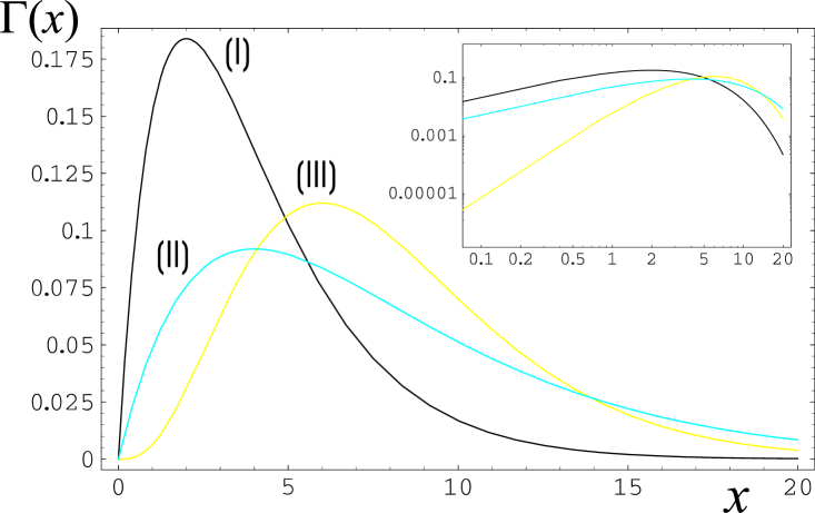
FIG. 1.: Representation of $\Gamma\left(x\right)$ $vs$ $x$ for some values of $\alpha$ and $\theta$. (I) - $\alpha=2$ and $\theta=2$;(II) - $\alpha=4$ and $\theta=2$; (III) - $\alpha=2$ and $\theta=4$. The inset presents the same curves, but in a $\log-\log$ scale.

II Introducing the generalised $\Gamma$-distribution

Let one now suppose that parameter $\theta$ in Eq. (3) is in fact a stochastic variable on time scale larger than the characteristic time scale $\gamma^{-1}$. This means that $p_{\alpha,\beta}\left(x\right)$ is, for this case, a conditional probability density function $p_{\alpha}\left(x\,|\,\beta\right)$. If the random process for $\beta$ is associatd with a SPDF, $\Pi\left(\beta\right)$, then the SPDF for $x$ variable, $P\left(x\right)$, is simply given by

$$P\left(x\right)=\int p_{\alpha}\left(x\,|\,\beta\right)\,\Pi\left(\beta\right)\,d\beta.$$ (8)

Among the various distributions for non-negative variables let one consider that $\beta$ is associated, itself, with a $\Gamma$-distribution,

$$P\left(x\right)=\int p_{\alpha}\left(x\,|\,\beta\right)\,\Pi\left(\beta\right)\,d\beta.$$ (9)

which can be associated to a microscopic equation similar to Eq. (6).

Calculating the integral presented in equation (8) one gets,

$$P\left(x\right)=\frac{\Gamma\left[\alpha+\lambda\right]\,\omega^{\alpha}}{\Gamma\left[\alpha\right]\,\Gamma\left[\lambda\right]}x^{\alpha-1}\,\left(1+\omega\,x\right)^{-\left(\alpha+\lambda\right)}.$$ (10)

Defining $\bar{\theta}=\frac{1}{\omega\,\left(\alpha+\lambda\right)}$ and $q=1+\frac{1}{\alpha+\lambda}$, Eq. (10) can be rewritten as,

$$P\left(x\right)=\frac{\Gamma\left[\frac{1}{q-1}\right]\,\left(\frac{q-1}{\bar{\theta}}\right)^{\alpha}}{\Gamma\left[\alpha\right]\,\Gamma\left[\frac{1}{q-1}-\alpha\right]}x^{\alpha-1}\left\{1-\left(1-q\right)\,\frac{x}{\bar{\theta}}\right\}^{\frac{1}{1-q}},$$ (11)

$$P\left(x\right)\equiv\frac{\Gamma\left[\frac{1}{q-1}\right]\,\left(\frac{q-1}{\bar{\theta}}\right)^{\alpha}}{\Gamma\left[\alpha\right]\,\Gamma\left[\frac{1}{q-1}-\alpha\right]}x^{\alpha-1}\exp_{q}\left[-\frac{x}{\bar{\theta}}\right],$$ (12)

which I will call the ${}_{q}\Gamma$-distribution. This kind of distribution was already verified, at least, for the distribution of traded volumes of stocks in financial markets [3]. For the limit $q\rightarrow 1$, the usual $\Gamma$-distribution is recovered, which corresponds to $\Pi\left(\beta\right)=\delta\left(\beta-\frac{1}{\theta}\right)$. Some examples of ${}_{q}\Gamma$-distribution are presented in Fig. 2,

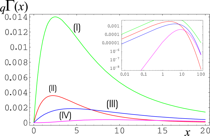
FIG. 2.: Representation of $\Gamma\left(x\right)$ $vs$ $x$ for some values of $\alpha$ and $\theta$. (I) - $q=1.2$, $\alpha=2$ and $\theta=2$; (II) - $q=1.1$, $\alpha=2$ and $\theta=2$;(III) - $q=1.1$, $\alpha=2$ and $\theta=4$; (IV) - $q=1.1$, $\alpha=4$ and $\theta=2$. The inset presents the same curves, but in a $\log-\log$ scale.

. The same form is presented in Figs. 7 and 8 of Ref. [3].

This problem of fluctuations in some intensive parameter of the dynamical equation(s) that describe(s) the evolution of a system [4] was recently studied by C. Beck in the context of Langevin equation with fluctuating temperature [5] and extended together with Eddie G.D. Cohen [6] who defined it as superstatistics (a statistic of statistics). This superstatistics presents a close relation to the non-extensive statistical mechanics framework based on the entropic form [7, 8],

$$S_{q}=\frac{1-\int\left[p\left(x\right)\right]^{q}\,dx}{q-1}.$$ (13)

For the problem of the distribution of traded volume of stocks in financial markets the presence of fluctuations in $\theta$, or the mean value of the scaled variable $\alpha\,x$, it is similar to the problem of the moving average in the analysis of the volatility useful in the reprodution of some empirical facts like the autocorrelation function and the so-called leverage efect, see e.g. Ref. [9].

REFERENCES

• [1] M.V. Jambunathan, Ann. Math. Stat. 25 (1954) 401;
• [2] H. Risken, The Fokker-Planck Equation - Methods of Solution and its Applications, $2^{nd}$ edition, (Springer-Verlag, Berlin) 1989;
• [3] R. Osório, L. Borland and C. Tsallis, Distributions of High-Frequency Stock-Market Observables in; M. Gell-Mann and C. Tsallis, Nonextensive Entropy - Interdisciplinary Applications (Oxford University Press, New York, 2004);
• [4] G. Wilk and Z. Włodarczyk, Phys. Rev. Lett. 84 (2000) 2770;
• [5] C. Beck, Phys. Rev. Lett. 87 (2001) 180601;
• [6] C. Beck and E.G.D. Cohen, Physica A 322 (2003)267;
• [7] C. Tsallis, J. Stat. Phys. 52 , 479 (1988). A regularly an updated bibliograhy on the subject is avaible at http://tsallis.cat.cbpf.br/biblio.htm;
• [8] M. Gell-Mann and C. Tsallis, Nonextensive Entropy - Interdisciplinary Applications (Oxford University Press, New York, 2004);
• [9] J. Perelló, J. Masoliver and J.P. Bouchaud, cond-mat/0302095 (preprint, 2003).