Spatial snowdrift game with myopic agents

Abstract

We have studied a spatially extended snowdrift game, in which the players are located on the sites of two-dimensional square lattices and repeatedly have to choose one of the two strategies, either cooperation (C) or defection (D). A player interacts with its nearest neighbors only, and aims at playing a strategy which maximizes its instant pay-off, assuming that the neighboring agents retain their strategies. If a player is not content with its current strategy, it will change it to the opposite one with probability $p$ next round. Here we show through simulations and analytical approach that these rules result in cooperation levels, which differ to large extent from those obtained using the replicator dynamics.

I Introduction

Understanding the emergence and persistence of cooperation is one of the central problems in evolutionary biology and socioeconomics MaynardSmith1995 ; Neumann1944 . In investigating this problem the standard framework utilized is evolutionary game theory Neumann1944 ; MaynardSmith1973 ; fudenberg . Especially two models, the Prisoner’s Dilemma Rapoport1965 ; Axelrod1981 ; Axelrod1988 and its variation, the snowdrift game MaynardSmith1973 ; Sugden1986 , have attracted most attention. In both games, the players can either cooperate for common good, or defect and exploit other players in attempt to gain benefits individually. In the Prisoner’s Dilemma, the precondition is that it pays off to be non-cooperative. Because of this, defection is the only evolutionarily stable strategy (ESS) in populations which are fully mixed, i.e. where each player interacts with any other player Smith1982 . However, several models which are extensions of the Prisoner’s Dilemma have proved to sustain cooperation. These models include those in which the players are assumed to have memory of the previous interactions Axelrod1984 , or characteristics that allow cooperators and defectors to distinguish each other Epstein1998 , or players are spatially distributed hauert ; Lindgren1997 ; Nowak1992 .

A typical spatial game is such where player-player interactions only take place within restricted neighborhoods on regular lattices Nowak1992 ; Doebeli1998 ; Szabo1998 ; Szabo2000 or on complex networks Zimmermann2004 . These games have been found to generate highly complex behavior and enable the persistence of cooperation. Regarding the latter, the opposite was recently seen in the case of the snowdrift game played on a two-dimensional lattice hauert , where the spatial structure resulted in decreased cooperator densities compared to the fully mixed “mean-field” case. This result was surprising, as intermediate levels of cooperation persist in unstructured snowdrift games, and the common belief has been that spatial structure is usually beneficial for sustained levels of cooperation.

In these studies the viewpoint has largely been that of biological evolution, as represented by the so-called replicator dynamics fudenberg ; Hofbauer1998 ; Nowak2004 , where the fraction of players who use high-payoff-strategies grow (stochastically) in the population proportionally to the payoffs. This mechanism can be viewed as depicting Darwinian evolution, where the fittest have the largest chance of survival and reproduction. Overall, the factors influencing the outcomes of these spatially structured games are (i) the rules determining the payoffs (e.g. Ref. fort2003 ), (ii) the topology of the spatial structure (e.g. Ref. Szabo2000 ), and (iii) the rules determining the evolution of each player’s strategy (e.g. Ref. Meyer1999 ; Traulsen2004 ). We have studied the effect of changing the strategy evolution rules (iii) in the two-dimensional snowdrift game similar to that discussed in Ref. hauert . In our version, the rules have been defined in such a way that changes in the players’ strategies represent player decisions instead of different strategy genotypes in the next evolutionary generation of players. Thus, the time scale of the population dynamics in our model can be viewed to be much shorter than evolutionary time scales. Instead of utilizing the evolution-inspired replicator dynamics, we have endowed the players with primitive “intelligence” in the form of local decision-making rules determining their strategies. We show with simulations and analytic approach that these rules result in cooperation levels which differ largely from those obtained using the replicator dynamics.

In this study we will concentrate on an adaptive snowdrift game, with agents interacting with their nearest neighbor agents on a two-dimensional square lattice. In what follows we first describe our spatial snowdrift model and then analyze its equilibrium states. Next we present our simulation results and finally draw some conclusions.

II Spatial Snowdrift Model

The snowdrift model can be illustrated with a situation in which two cars are caught in a blizzard and there is a snowdrift blocking their way. The cars are equipped with shovels, and the drivers have two choices: either start shoveling the road open or remain in the car. If the road is cleared, both drivers gain the benefit $b$ of getting home. On the other hand, clearing the road requires some work, and cost $c$ can be assigned to it ($b>c>0$). If both drivers are cooperative and willing to shovel, this workload is shared between them, and both of them gain total benefit of $R=c-b/2$. If both choose to defect, i.e. remain in their cars, neither one gets home and thus both obtain zero benefit $P=0$. If only one of the drivers shovels, both get home, but the defector avoids the cost and gains benefit $T=b$, whereas the cooperator’s benefit is reduced by the workload, i.e. $S=b-c$.

The above described situation can be presented with the bi-matrix gibbons (Table 1), where

$$T>R>S>P.$$ (1)

In case of the so called one-shot game, each player has two available strategies, namely defect (D) or cooperate (C). The players choose their strategies simultaneously, and their individual payoffs are given by the appropriate cell of the bi-matrix. By convention, the payoff to the so-called row player is the first payoff given, followed by the payoff of the column player. Thus, if for example player 1 chooses D and player 2 chooses C, then player 1 receives the payoff T and player 2 the payoff S.

The best action depends on the action of the co-player such that defect if the other player cooperates and cooperate if the other defects. A simple analysis shows that the game does not have stable evolutionary strategy Hofbauer1998 , if the agents use only pure strategies, i.e., they can choose either to cooperate or to defect with probability one, but they are not allowed to use a strategy which mixes either of these actions with some probability $q\in(0,1)$. This leads to stable existence of cooperators and defectors in well-mixed populations hauert .

Table 1: Snowdrift game. Player 1 chooses an action from the rows and player 2 from the columns. By convention, the payoff to the row player is the first payoff given, followed by the payoff of the column player.

	D	C
D	P, P	T, S
C	S, T	R, R

In order to study the effect of spatial structure on the snowdrift game, we set the players on a regular two-dimensional square lattice consisting of $m$ cells. We adopt the notation of Ref. (schweitzer ) and identify each cell by an index $i=1,\ldots,m$ which also refers to its spatial position. Each cell, representing a player, is characterized by its strategy $s_{i}$, which can be either to cooperate ($s_{i}=1$) or to defect ($s_{i}=0$). The spatio-temporal distribution of the players is then described by $S=(s_{1},\ldots,s_{m})$ which is an element of a $2^{m}$ dimensional hypercube. Then every player – henceforth called an agent – interacts with their $n$ nearest neighbors. We use either the Moore neighborhood in which case each agent has $n=8$ neighbors, in N,NE,E,SE,S,SW,W and NW, or the von Neumann neighborhood in which case each agent has $n=4$ neighbors, in N,E,S and W compass directions adachi . We require that an agent plays simultaneously with all its $n$ neighbors, and define the payoffs for this $(n+1)-player$ game such that an agent $i$ who interacts with $n_{c}^{i}$ cooperators and $n_{d}^{i}$ defectors, $n_{c}^{i}+n_{d}^{i}=n$, gains a benefit of

$$u_{i}(s_{i}=0) = n_{c}^{i}T+n_{d}^{i}P$$ (2)

$$u_{i}(s_{i}=1) = n_{c}^{i}R+n_{d}^{i}S,$$ (3)

from defecting or cooperating, respectively.

For determining their strategies, the agents are endowed with primitive decision-making capabilities. The agents retain no memory of the past, and are not able to predict how the strategies of the neighboring agents will change. Every agent simply assumes that the strategies of other agents within its neighborhood remain fixed, and chooses an action that maximizes its own payoff. In this sense the agents are myopic. The payoff is maximized, if an agent (a) defects when $u_{i}(0)>u_{i}(1)$, and (b) cooperates when $u_{i}(1)>u_{i}(0)$. If (c) $u_{i}(0)=u_{i}(1)$ the situation is indifferent. Using Eqs. (2) and (3) we can connect the preferable choice of an agent and the payoffs of the game. Let us denote

$$\frac{1}{r}=1+\frac{S-P}{T-R}.$$ (4)

Then, if

$$\frac{n_{c}^{i}}{n} > 1-r\textrm{ defecting is profitable, or if}$$ (5)

$$\frac{n_{c}^{i}}{n} < 1-r\textrm{ cooperating is profitable, or if}$$ (6)

$$\frac{n_{c}^{i}}{n} = 1-r\textrm{ choices are indifferent}.$$ (7)

Thus, for each individual agent, the ratio $r$ determines a following decision-boundary

$$\theta=n(1-r),$$ (8)

which depends on the neighborhood size $n$ and the “temptation” parameter $r$. Because $r$ is determined only by the differences $T-R$ and $S-P$, we can fix two of the payoff values, say $R=1$ and $P=0$. Based on the above, we define the following rules for the agents:

1. If an agent $i$ plays at time $t$ a strategy $s_{i}(t)\in\{0,1\}$ for which $u_{i}(s_{i})\geq u_{i}(1-s_{i})$, then at time $t+1$ the agent plays $s_{i}(t+1)=s_{i}(t)$.

2. If an agent $i$ plays at time $t$ a strategy $s_{i}(t)\in\{0,1\}$ for which $u_{i}(s_{i})<u_{i}(1-s_{i})$, then at time $t+1$ the agent plays $s_{i}(t+1)=1-s_{i}(t)$ with probability $p$, and $s_{i}(t+1)=s_{i}(t)$ with probability $1-p$.

Hence, the strategy evolution of an individual agent is determined by the current strategies of the other agents within its neighborhood, with the parameter $p$ acting as a “regulator” which moderates the rate of changes.

III Equilibrium states

A spatial game is in stable state or equilibrium if retaining the current strategy is beneficial for all the agents fudenberg . There can be numerous equilibrium configurations, depending on the temptation parameter $r$, geometry and size of the $n$-neighborhood, and the size and boundary conditions of the lattice upon which the game is played. An aggregate quantity of particular interest is the fraction of cooperators $F_{c}$ in the whole population (or, equivalently, that of the defectors $F_{d}$). Below, we derive limits for $F_{c}$, first in a “mean-field” picture based cooperator densities within neighborhoods and then by investigating local neighborhood configurations.

III.1 Mean-field limits for cooperator density

Without detailed knowledge of local equilibrium configurations we can already derive some limits for the fraction of cooperators in equilibrium. Let us consider a square lattice with $m=L\times L$ cells with periodic boundary conditions, where $L$ is the linear size of the lattice, and assume that $k$ cells are occupied by cooperators. We denote by $a_{j}$ the number of those agents who have $j$ cooperators each in their $n$-neighborhood, excluding the agents themselves, and denote the local density of cooperators in such neighborhoods by $f_{c}=j/n$. Hence, the total amount of cooperators $k$ can be written in terms of the densities as follows

$$k=\sum_{j=0}^{n}a_{j}f_{c}=\sum_{j=0}^{n}a_{j}\frac{j}{n}.$$ (9)

From Eqs. (5)-(7) we can infer that a cooperator will retain its current strategy, if it has at most $c$ cooperators in its $n$-neighborhood, where $c$ is the integer part of $\theta=n(1-r)$. Similarly, a defector will remain a defector if it has more than $c$ cooperators in its neighborhood. Thus, in equilibrium, all agents having $j\leq c$ cooperators in their neighborhood are likewise cooperators, and thus $\sum_{j=0}^{c}a_{j}=k$. We denote by $\left<f_{c|c}\right>=\frac{1}{k}\sum_{j=0}^{c}a_{j}\frac{j}{n}$ the average density of cooperators as the nearest neighbors of cooperators. Similarly, $\left<f_{c|d}\right>$ denotes the average density of cooperators as the nearest neighbors of defectors, i.e. $\left<f_{c|d}\right>=\frac{1}{m-k}\sum_{j=c+1}^{n}a_{j}\frac{j}{n}$. Then we can write Eq. (9) as

$$k=k\left<f_{c|c}\right>+(m-k)\left<f_{c|d}\right>.$$ (10)

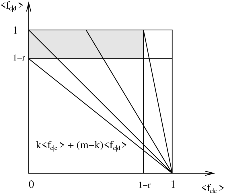
Figure 1: In equilibrium the average density of cooperators in the nearest neighborhood of defectors must be $1-r\leq\left<f_{c|d}\right>\leq 1$ and in the nearest neighborhood of cooperators $0\leq\left<f_{c|c}\right>\leq 1-r$ (shaded area). If the total number of players in the lattice is $m$, the lines $k\left<f_{c|c}\right>+(m-k)\left<f_{c|d}\right>=k$ depict the identity of $k$ cooperators in the lattice. Equilibrium is not possible, if the fraction of cooperators $F_{c}=k/m$ is such that the lines do not pass through the shaded area.

The density $f_{c|c}$ of cooperators around each cooperator is bounded: $f_{c|c}\geq 0$, $f_{c|c}\leq c/n$, and as $c\leq\theta=n(1-r)$, the relation $0\leq\left<f_{c|c}\right>\leq 1-r$ holds for the average density. Similarly, the density of cooperators around each defector $f_{c|d}$ can be at most $1$ and is at least $(1-r)$, and thus the average density $1-r\leq\left<f_{c|d}\right>\leq 1$. Using these relations together with Eq. (10) we obtain the following limits for the density of cooperators $F_{c}=k/m$ in the whole agent population (see also Fig. 1):

$$\frac{1-r}{2-r}\leq F_{c}\leq\frac{1}{r+1}.$$ (11)

III.2 Local equilibrium configurations

In the above derivation we ignore how the strategies can actually be distributed in the lattice. Hence, it is of interest to examine possible local equilibrium configurations of the player strategies. Again, Eqs. (5)-(7) tell us how many cooperative neighbors each defector or cooperator can have in the equilibrium state. The number of cooperators around each agent depends on the value of the temptation parameter $r$, and for a given value of $r$ the lattice has to be filled such that these conditions hold for the neighborhood of each agent. In a lattice with periodic boundary conditions, the lattice size $m=L_{X}\times L_{Y}$ and the neighborhood size $n$ obviously have an effect on the elementary configurations. Hence, we restrict ourselves to infinite-sized lattices, filled by repeating elementary configuration blocks, and look for the resulting limits on the cooperator density $F_{c}$. Note that these conclusions also hold for finite lattices with periodic boundary conditions, if $L_{X}$ and $L_{Y}$ are integer multiples of $X$ and $Y$, respectively, where $X\times Y$ is the elementary block size. Here, we will restrict the analysis to the case of the Moore neighborhood with $n=8$.

Table 2: Limits for the equilibrium fraction of cooperators based on repeating elementary configuration blocks. When $r_{l}<r<r_{u}$, the number of cooperators in each defector’s neighborhood $N_{c|d}$ must be at least $9-i$ and the number of cooperators in each cooperator’s neighborhood $N_{c|c}$ at most $8-i$. Considering possible repeating configuration blocks which fulfill these conditions, we obtain lower limits $F_{c,L}$ and upper limits $F_{c,U}$ for the density of cooperators.

i	$r_{l}$	$r_{u}$	$N_{c|d}\geq$	$N_{c|c}\leq$	$F_{c,L}$	$F_{c,U}$
1	$0$	$1/8$	8	7	$3/4$	$8/9$
2	$1/8$	$2/8$	7	6	$2/3$	$4/5$
3	$2/8$	$3/8$	6	5	$1/2$	$2/3$
4	$3/8$	$4/8$	5	4	$1/2$	$2/3$
5	$4/8$	$5/8$	4	3	$4/9$	$1/2$
6	$5/8$	$6/8$	3	2	$1/3$	$1/2$
7	$6/8$	$7/8$	2	1	$2/9$	$1/3$
8	$7/8$	$8/8$	1	0	$1/9$	$1/4$

Figure 2: Examples of elementary configuration blocks which can be repeated without overlap to fill an infinite lattice, for various values of $r$. The numbering refers to $i$ in Table 2. A black cell denotes a defector while an empty cell denotes a cooperator. For a particular number the lower limit of density is obtained by filling the lattice with the blocks on the left, and the upper by using the blocks on the right.

As an example, consider the local configurations when $r=0.1$, and hence the decision boundary value $\theta=n(1-r)=7.2$. Thus, from Eqs. (5)-(7) one can infer that in equilibrium all defectors should have more than $7.2$ cooperators in their Moore neighborhoods. Because the number of cooperating neighbors can take only integer values, this means that every one of the $n=8$ neighbors of a defector should be a cooperator. On the other hand, from Eqs. (5)-(7) we see that the density $f_{c|c}$ of cooperators around each cooperator should be less than $1-r$, i.e. they should have at most $c=7$ cooperators in their Moore neighborhood. The smallest repeated elementary block fulfilling both conditions is a $2\times 2$-square with one defector – when the lattice is filled with these blocks, the cooperator density equals $F_{c}=3/4$ (see Fig. (2), case 1, left block). On the other hand, both requirements are likewise fulfilled with a repeated $3\times 3$-square, where the central cell is a defector and the rest are cooperators, resulting in the cooperator density of $F_{c}=8/9$. This configuration is illustrated in Fig. (2), as case 1, right block.

By continuing the analysis of elementary configuration blocks in similar fashion for different values of $r$, we obtain lower and upper limits for the fraction of cooperators, which are listed in Table 2. The corresponding elementary configuration blocks are depicted in Fig. (2). The table is read so that when the value of the temptation parameter is within the interval $r_{l}<r<r_{u}$, the number of cooperators in each defector’s neighborhood $N_{c|d}$ must be at least $9-i$ and the number of cooperators in each cooperator’s neighborhood $N_{c|c}$ can be at most $8-i$. Here $r_{l}=(i-1)/8$, $r_{u}=i/8$ and $i=1,\ldots,8$ These conditions are those of Eqs. (5)-(7) and they are fulfilled by the configuration blocks depicted in Fig. (2), for which the minimum and maximum densities of cooperators are $F_{c,L}$ and $F_{c,U}$.

IV Simulation results

We have studied the above described spatial snowdrift model with discrete time-step simulations on a $m=100\times 100$-lattice with periodic boundary conditions. We have specifically analyzed the behavior of the cooperator density $F_{c}$, and equilibrium lattice configurations. In the simulations, the lattice is initialized randomly so that each cell contains a cooperator or defector with equal probability. However, biasing the initial densities toward cooperators or defectors was found to have no considerable effect on the outcome of the game. We have simulated the game using both the Moore and the von Neumann neighborhoods with $n=8$ and $n=4$ nearest neighbors, respectively. In the simulations we update strategies of the agents asynchronously adachi with the random sequential update scheme, so that during one simulation round, every agent’s strategies are updated in random order. In the following, the time scale is defined in terms of these simulation rounds.

First, we have studied the development of the cooperator density $F_{c}$ as a function of time. As expected, the probability $p$ of discontent agents changing their strategies plays the role of defining the convergence time scale only, as in the long run $F_{c}$ converges to a stable value irrespective of $p$. This is depicted in Fig. 3, which shows $F_{c}$ as function of time for several values of $p$ and two different values of the temptation $r$. In these runs, we have used the Moore neighborhood, i.e. $n=8$. In all the studied cases, $F_{c}$ turns out to converge quite rapidly to a constant value, $F_{c}\sim 0.7$ for $r=0.2$ and $F_{c}\sim 0.3$ for $r=0.8$.

It should be noted that $F_{c}$ does not have to converge to exactly the same stable value for the same $r$; even if the game is considered to be in equilibrium, there can be some variance in $F_{c}$, which is also visible in Fig. 3. However, the value of $F_{c}$ was found to eventually remain stable during individual runs, i.e. no oscillations were detected.

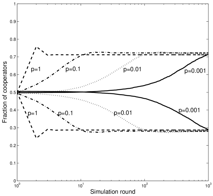
Figure 3: Dynamics of the fraction of cooperators $F_{c}$. The upper curves that converge to $F_{c}\sim 0.7$ are for $r=0.2$, and the lower curves that converge to $F_{c}\sim 0.3$ are for $r=0.8$. In both cases the probability of being discontent is varied as $p=1,0.1,0.01,0.001$ from left to right, and the lattice size is $m=100x100$.

Next, we have studied the average equilibrium fraction of cooperators $\left<F_{c}\right>$ in the agent population as function of the temptation parameter $r$. We let the simulations run for 500 rounds (with $p=0.1$), and averaged the fraction of cooperators for the subsequent 500 rounds. In all cases, the fraction had already converged before the averaging rounds. Fig. (4) shows the results for the von Neumann neighborhood ($n=4$), illustrated as the squares. The dotted lines indicate the upper and lower limits of Eq. (11), and the dashed diagonal line is $F_{c}=1-r$, corresponding to the fraction of cooperators in the fully mixed case fudenberg ; hauert ; Hofbauer1998 . The fraction of cooperators $\left<F_{c}\right>$ is seen to follow a stepped curve, with steps corresponding to $r=i/n$, where $i=0,\ldots,n$. This is a natural consequence of Eqs. (5)-(7), where the decision boundary $\theta=n(1-r)$ can take only discrete values. A similar picture is given for the Moore neighborhood ($n=8$) in the middle panel of Fig. (5). Furthermore, in the middle panel of Fig. (5) the values of $F_{c}$ fall between the limits given in Table 2 for all $r$ as shown with solid lines.

In both cases (i.e. with Moore and von Neumann neighborhoods) cooperation is seen to persist during the whole range $r=[0,1]$. This result differs largely from the $F_{c}(r)$-curves of the spatial snowdrift game with replicator dynamics hauert , where the fraction of cooperators vanished at some critical $r_{c}$. Hence, we argue that no conclusions on the effect of spatiality on the snowdrift game can be drawn without taking into consideration the strategy evolution mechanism; local decision-making in a restricted neighborhood yields results which are different from those resulting from the evolutionary replicator dynamics.

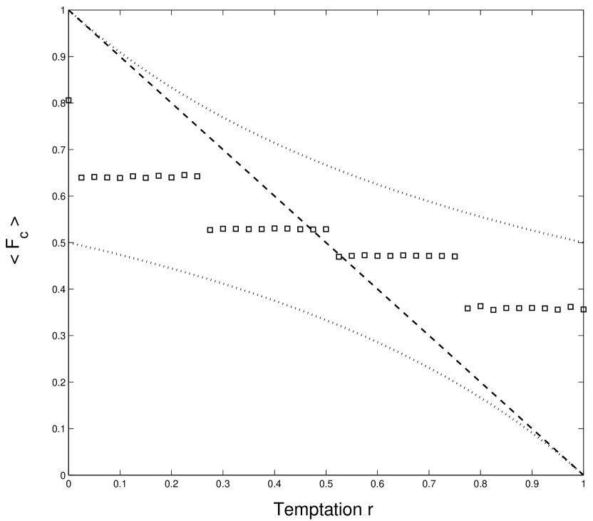
Figure 4: Average fraction of cooperators $\left<F_{c}\right>$ versus the temptation $r$ (squares), simulated on a $100\times 100$ lattice with $p=0.1$ using the von Neumann neighborhood. The values for $\left<F_{c}\right>$ are averages over 500 simulation rounds, where the averaging was started after 500 initial rounds to guarantee convergence. The dotted lines depict the upper and lower limits for $F_{c}$ of Eq. (11). The dashed diagonal line is $1-r$.

We have also studied the equilibrium lattice configurations for various values of $r$. Fig. (5) depicts the central part of the $100\times 100$-lattice after 1000 simulation rounds using the Moore neighborhood and $p=0.1$, with white pixels corresponding to cooperators and black pixels to defectors. The values of $r$ have been selected so that the equilibrium situation corresponds to each plateau of $\left<F_{c}\right>$ illustrated in the central panel.

The observed configurations are rather polymorphic, and repeating elementary patterns like those in Fig. (2) are not seen. This reflects the fact that the local equilibrium conditions can be satisfied by various configurations; the random initial configuration and the asynchronous update then lead to irregular-looking equilibrium patterns, which vary between simulation runs. The patterns seem to be most irregular when $r$ is around 0.5; this is because then the equilibrium numbers of cooperators and defectors are close to each other, and the ways to assign strategies within local neighborhoods are most numerous. To be more exact, there are $8\choose i$ ways to distribute $i$ cooperators in the $8$-neighborhood, and if e.g. $3/8<r<4/8$, $i$ is at least $4$ and at most $5$, maximizing the value of the binomial coefficient. Hence, the ways of filling the lattice with these neighborhoods in such a way that the equilibrium conditions are satisfied everywhere are most numerous as well.

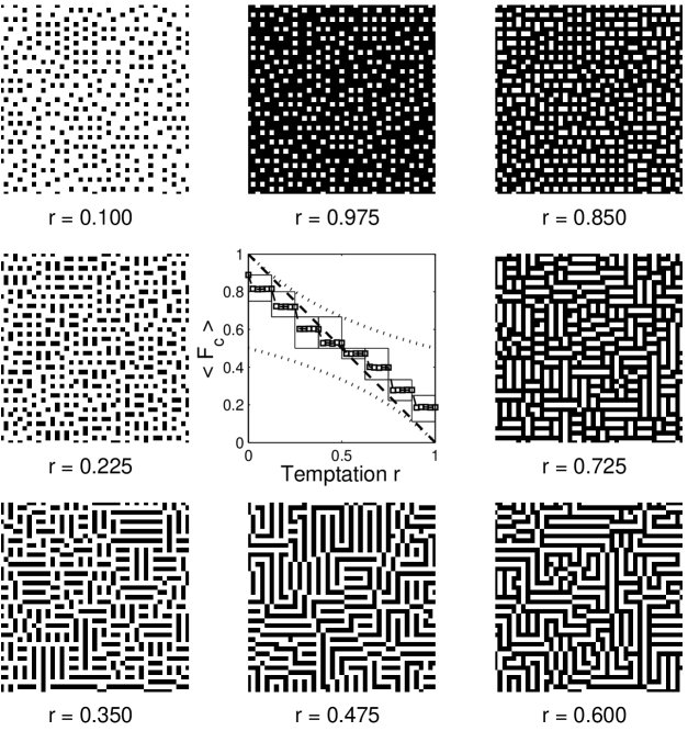
Figure 5: Example equilibrium configurations of defectors and cooperators on a $m=100\times 100$ lattice for various values of $r$ when the Moore neighborhood is used. The configurations were recorded after $T=1000$ simulation rounds. Only the middle part of the lattice is shown for the sake of clarity. The middle panel depicts the average fraction of cooperators $\left<F_{c}\right>$ in the whole population as a function of the temptation $r$ (squares), together with the upper and lower limits of Eq. (11) (dotted lines) and the limits of Table 2 (solid lines). The values of $\left<F_{c}\right>$ are averages over the last 500 simulation rounds and the dashed diagonal line is $F_{c}=1-r$, corresponding to the fraction of cooperators in the fully mixed case fudenberg ; hauert ; Hofbauer1998 .

V Summary and conclusions

We have presented a variant of the two-dimensional snowdrift game, where the strategy evolution is determined by agent decisions based on the strategies of other players within its local neighborhood. We have analyzed the lower and upper bounds for equilibrium cooperator densities with a mean-field approach as well as considering possible lattice-filling elementary configuration blocks. We have also shown with simulations that this game converges to equilibrium configurations with constant cooperator density depending on the payoff parameters, and that these densities fall within the derived limits. Furthermore, the strategy configurations in the equilibrium state display interesting patterns, especially for intermediate temptation parameter values.

Most interestingly, the equilibrium cooperator densities differ largely from those resulting from applying the replicator dynamics hauert . With our strategy evolution rules, cooperation persists through the whole temptation parameter range. This illustrates that one cannot draw general conclusions on the effect of spatiality on the snowdrift game without taking the strategy evolution mechanisms into consideration – this should, in principle, apply for other spatial games as well. Care should especially be taken when interpreting the results of investigations on such games: the utilized strategy evolution mechanism should reflect the system under study. We argue that especially when modeling social or economic systems, there is no a priori reason to assume that generalized conclusions can be drawn based on results using the evolution inspired replicator dynamics approach, where high-payoff strategies get copied and “breed” in proportion to their fitness. As we have shown here, local decision-making with limited information (neighbor strategies are known payoffs are not) can result in different outcome.

References

- (1) J. Maynard Smith and E. Szathmáry, The Major Transitions in Evolution (W.H. Freeman, Oxford, UK, 1995).
- (2) J. von Neumann and O. Morgenstern, Theory of Games and Economic Behaviour (Princeton University Press, 1944).
- (3) J. Maynard Smith and G. Price, Nature 246 (1973) 15-18.
- (4) D. Fudenberg and D. K. Levine, The Theory of Learning in Games (The MIT Press, 1998).
- (5) A. Rapoport and A. Chammah, Prisoner’s Dilemma (University of Michigan Press, Ann Arbor, 1965).
- (6) R. Axelrod and W.D. Hamilton, Science 211, (1981) 1390-1396.
- (7) R. Axelrod and D. Dion, Science 242, (1988) 1385-1390.
- (8) R. Sugden, The Economics of Rights, Co-operation and Welfare (Blackwell, Oxford, UK, 1986).
- (9) J.M. Smith, Evolution and the theory of games (Cambridge University Press, Cambridge, UK, 1982).
- (10) R. Axelrod, The evolution of cooperation, (Basic Books, New Yourk, 1984).
- (11) J. N. Epstein, Complexity 4(2), (1998) 36-48.
- (12) C. Hauert and M. Doebell, Nature 428, (2004) 643-646.
- (13) K. Lindgren, Evolutionary Dynamics in Game-Theoretic Models in The Economy as an Evolving Complex System II (Addison-Wesley, 1997) 337-367.
- (14) M. A. Nowak and R. May, Nature 359 (1992) 826-829.
- (15) M. Doebeli and N. Knowlton, Proc. Natl Acad. Sci USA 95 (1998) 8676-8680.
- (16) G. Szabó and C. Toke, Phys. Rev. E 58 (1998) 69-73.
- (17) G. Szabó, T. Antal, P. Szabó and M. Droz, Phys. Rev. E 62 (2000) 1095-1103.
- (18) M. G. Zimmermann, V. M. Eguíluz and M. San Miguel, Phys. Rev. E 69 (2004) 065102.
- (19) J. Hofbauer and K. Sigmund, Evolutionary games and population dynamics, (Cambridge University Press, Cambridge, UK, 1998).
- (20) M. A. Nowak and K. Sigmund, Science 303 (2004) 793-799.
- (21) H. Fort, Phys. Rev. E (2003) 68 026118.
- (22) D. A. Meyer, Phys.Rev.Lett. 82 (1999) 1052-1055.
- (23) A. Traulsen, T. Röhl and H.G.Schuster, Phys.Rev.Lett. 93 (2004) 028701.
- (24) R. Gibbons, Game Theory for Applied Economists, (Princeton University Press, 1992).
- (25) F. Schweitzer, L. Behera and H. Mühlenbein, Advances in Complex Systems 5 (2002) 269-299.
- (26) S. Adachi, F. Peper and J. Lee, Journal of Statistical Physics 114 (2004) 261-289.