Neural network prediction of geomagnetic activity: a method using local Hölder exponents
Abstract
Local scaling and singularity properties of solar wind and geomagnetic time series were analysed using Hölder exponents . It was shown that in analysed cases due to multifractality of fluctuations changes from point to point. We argued there exists a peculiar interplay between regularity / irregularity and amplitude characteristics of fluctuations which could be exploited for improvement of predictions of geomagnetic activity. To this end layered backpropagation artificial neural network model with feedback connection was used for the study of the solar wind - magnetosphere coupling and prediction of geomagnetic index. The solar wind input was taken from principal component analysis of interplanetary magnetic field, proton density and bulk velocity. Superior network performance was achieved in cases when the information on local Hölder exponents was added to the input layer.
1 Introduction
One of the goals of solar-terrestrial physics is to predict the response of magnetosphere-ionosphere system to highly variable conditions in the solar wind (SW). The question of solar wind-magnetosphere coupling (SWMC) can be studied by means of input-output modelling. Linear input-output techniques (or linear prediction filtering) describe the SWMC by a linear moving-average (MA) filter assuming that the convolution of a time-invariant transfer function (TF), with an earlier SW input can predict the magnetospheric output represented by time series of geomagnetic indices [Iyemori et al.(1979), Bargatze et al.(1985), McPherron et al.(1988)]. The TF characterizes the magnetospheric response and can be estimated directly from data provided that a sufficiently large number of input-output pairs is available. In fact, [Bargatze et al.(1985)] using the input-output data ( - solar wind velocity, - interplanetary magnetic field component, - auroral zone geomagnetic index) have shown that the linear MA filters can identify two different regimes in which SW energy is dissipated within the magnetosphere (directly driven and loading-unloading regimes). At the same time, the best linear MA filters do not predict the geomagnetic output precisely, unless strongly varying filter parameters are considered in each case of activity level separately [Blanchard and McPherron(1994)]. Different levels of geomagnetic activity and the nonlinearity of the SWMC were then treated by nonlinear MA filters [Price et al.(1994), Vassiliadis et al.(1995)] using the assumption that the geomagnetic activity is a nonlinear function of the solar wind input. Actually, local linear (that is nonlinear) MA filters were used, which represent a linear approximation of the nonlinear system. Nonlinear MA filters proved to be better predictors of geomagnetic response as the linear ones, but the internal dynamics of the magnetosphere and the additional influence of it on the geomagnetic response itself (a feedback) was more explicitly considered within the frame of state-input space models [Vassiliadis et al.(1995)]. Here the prediction of magnetospheric states is made within a common input (solar wind) - output (geomagnetic data) phase space and the local linear (nonlinear) approximation is given by an evolution of the nearest neighbours of a phase space point. [Vassiliadis et al.(1995)] found that in comparison with linear state-input models (global aproximation) the nonlinear state-input models (local approximation based on nearest neighbours) give better predictions of geomagnetic activity.
An alternative to the above MA filters is represented by artificial neural networks (ANN) which are global nonlinear functions. Elman recurrent ANN was used by [Munsami (2000)] to model SW forcing of the westward auroral electroject and the storm-time ring current. In predicting geomagnetic activity their performance was similar to that of linear filters [Hernandez et al.(1993)]. Significantly better performance was achieved by gated ANNs that accounted for different levels of activity. [Weigel et al.(1999)] used three individual ANNs for modelling low, medium and high activity levels using data from database of [Bargatze et al.(1985)]. The outputs of these ANNs together with past geomagnetic outputs were used to train the gate network. It was shown by [Weigel et al.(1999)] and [Weigel(2000)] that the gated architecture give significantly better predictions as the ungated one or the ARMA system reported by [Hernandez et al.(1993)]. Obviously, the gated ANN architecture resembles the state-input space model of [Vassiliadis et al.(1995)] giving account for changing activity levels. Local linear filters can be calculated in a neighbour of any point in state-input space, the gated ANN, however, uses only three levels of activity.
In this paper we propose a method which allows to consider the changing level of SW fluctuations. Instead of building a more structured gated ANN architecture we use the extra information on local scaling characteristics of properly introduced measure which can be estimated directly from a time series. Multifractals exhibit time-dependent scaling laws and hence allow a description of irregular phenomena that are localized in time. Multifractal scaling characteristics of geomagnetic fluctuations were studied by [Consolini et al.(1996)] and [Vörös(2000)]. [Jankovičová et al.(2001)] using multilayer feed-forward ANN have shown that the information on multifractal characteristics of geomagnetic data put to the input enhanced the performance of their ANN in reconstructing AE-index time series from geomagnetic observatory data. The inclusion of multifractality, however, somewhat amplified the noise component in this case. We expect that the inclusion of the scaling characteristics of solar wind and geomagnetic fluctuations to the ANN modelling of SWMC offers a way for considering essential local information on rapid changes, irregularities and intermittence not considered enough hitherto. Intermittence of SW and geomagnetic fluctuations was not built into nonlinear filter or ANN models. Notwithstanding that SW fluctuations proved to be strongly intermittent [Burlaga(1991), Carbone(1994), Marsch et al.(1996), Tu et al.(1996), Bruno et al.(1999)] and also both nonlinear magnetotail theories [Chang(1999), Chapman et al.(1998), Klimas et al.(2000)] and experimental works [Consolini et al.(1996), Borovsky et al.(1997), Consolini and De Michelis(1998), Consolini and Lui(1999), Vörös(2000), Kovács et al.(2001), Watkins et al.(2001)] predict or confirm the presence of scalings, multifractality and intermittence within the magnetosphere. Though there exist competing theoretical concepts regarding the underlying physical mechanisms which may or may not produce the observed scalings [Freeman et al.(2000), Antoni et al.(2001)] these considerations have no effect on our analysis. We simply ask what are the scaling characteristics of fluctuations and how can this information improve our ability to predict geomagnetic activity using ANNs.
2 Data analysis methods
2.1 Local scaling characteristics: the Hölder exponents
We consider the accumulated amount of signal energy within a window . The signal energy within a window is computed as a sum of the squared amplitudes of time series through
| (1) |
and
| (2) |
where represents a time series, is the total number of data points. The distribution of in time is considered to be a measure which may also appear as singular. Mathematically, a measure can be characterized by its density. An erratic behaviour appears in the absence of a density for a singular measure. Generally, singular distributions can be characterized locally by the so-called singularity or Hölder exponents [Halsey et al.(1986), Muzy et al.(1994), Véhel and Vojak(1998)]. Loosely speaking, the exponent quantify the degree of regularity or irregularity (singularity) in a distribution or a function in a point . Usually, the measure within a window scales as . Therefore, can be estimated by a regression method using
| (3) |
taking different window lengths . For a monofractal for all , while in a case of multifractal measure (non-uniform distribution) changes from point to point (non-stationarity). For instance, fractional Brownian motion or continuous Itô processes represent self-affine fluctuations governed by a single Hölder exponent. The global distribution of singularity exponents for geomagnetic fluctuations was studied by [Consolini et al.(1996)] and [Vörös(2000)]. It was shown that on the time scale of substorms and storms geomagnetic fluctuations seem to be analogous to the simple multiplicative -model which describes energy cascade processes in turbulent flows. This model explains how a specific energy flux introduced on large scales to a flow can lead to non-homogeneous, intermittent energy distributions on small scales. On this basis we expect that in case of homogeneous energy transfer rate between scales with no intermittency effects, the above defined distribution will be stationary and for all . Otherwise, indicate irregularities, sharp variations around , while is found in regions where events are more regular [Riedi and Véhel(1997)]. In case of multifractal processes changes from point to point, which usually makes difficult the numerical estimation of ’s. A number of papers deals with this question [Muzy et al.(1994), Jaffard and Meyer(1996), Mallat and Hwang(1992), Véhel and Vojak(1998)]. Though the Hölder exponents do not characterize the local regularity properties of a signal completely [Guiheneuf et al.(1998)], we are going to use the simple relation (3) to show that even a rough estimation of local scaling characteristics of the signal may enhance the performance of ANNs. We note that a running numerical estimate of may fluctuate sharply for other, from multifractality different, nonstationary processes.
2.2 ANN description
A layered backpropagation ANN model [Rumelhart et al.(1986), Kröse and Smagt(1996)] with feedback connection from output layer to input layer was constructed. The output-input layer connection makes the output history to be an ordinary input unit in training process. The output of the model can be expressed in the form
| (4) |
where denotes the time series; the two inputs equal and ; the history; the time resolution ( h); the weights between input and hidden layers; the weights between hidden and output layers; the biases of the layers; the number of hidden units; and the nonlinear activation function. In our model are the hyperbolic tangent and the linear activation functions and . The performance of the ANN model was evaluated through root mean squared error () and correlation coefficient ()
| (5) |
| (6) |
where denotes an actual output, its mean value and a one-step ahead prediction of ANN, its mean value; is their length; and are the standard deviations of and .
3 Data analysis
In this paper we are going to predict the index one hour in advance using the layered backpropagation ANN model with feedback connection. Prior to that, we show several examples which demonstrate that the Hölder exponents estimated by Equation 3 provide local characteristics of the analysed time series sensitive enough to capture the necessary information on the abrupt changes and activity levels.
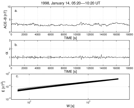
Figure 1a shows interplanetary magnetic field (IMF) variations registered by the ACE satellite which is continuously monitoring the SW at the Earth-Sun Lagrange point. The time resolution is 16 s and 5 hours of data is shown from January 14, 1998, 05:20 UT. This is a time period of very low activity level with mean value of IMF ACE fluctuations of 3 nT. The Hölder exponents estimated within variable window length s at each point are depicted in Figure 1b. It is visible that fluctuates around its mean value , which means that the measure is almost uniformly distributed. The energy content of the signal , and its scaling with window length, that is , is shown in a log-log plot in Figure 1c.
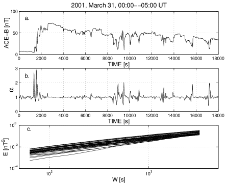
In contrast with Figure 1, Figure 2 shows a more disturbed period of IMF ACE variations from March 31, 2001 from 00:00 to 05:00 UT. The mean value of is 43 nT. Large departures from are present (Figure 1b), mainly within time periods of enhanced fluctuations. These periods are characterized by sudden increase of regularity () followed by periods of low regularity () or vice-versa.
In fact, appears to be a sensitive indicator of fluctuations which may occur during periods of enhanced IMF amplitudes, however, when the fluctuations cease, the values of return to , independently on the actual amplitudes. A good example of it is visible within the time interval s in Figures 2 a, b, where nT and . Moreover, the local fluctuations of around seem to be larger when the gradient of increases, but it is not always valid (not shown). There is also a clear difference between the scalings in Figure 1c and 2c.
We conclude that, besides the amplitude of magnetic field variations, the local scaling properties of signal described by Hölder exponents (Equation 3) may represent an essential piece of information the consideration of which would allow a better prediction of future geomagnetic activity.
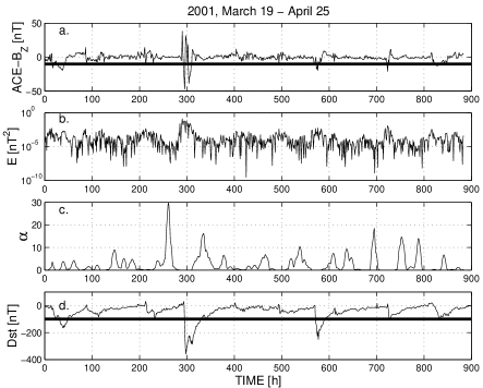
Other examples of longer period data sets (from March 19 to April 25, 2001) are depicted in Figure 3. This time, IMF from ACE satellite and the index are considered with time resolution of 1 hour. The thick line in Figure 3a corresponding to nT highlights periods of enhanced SWMC.
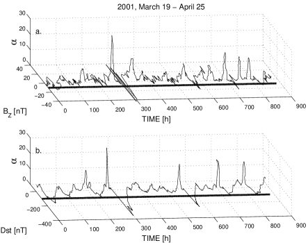
[Gonzalez and Tsurutani(1987)] have shown that the interplanetary causes of intense magnetic storms ( nT) are long duration ( h) large and negative ( nT) events associated with interplanetary duskward electric fields . Comparison of Figures 3a, d shows an agreement with the above criteria, that is, long duration negative IMF events occur together with intense magnetic storms. Horizonthal thick line corresponds to the limit of nT in Figure 3d. Figure 3b shows the normalized measure and the estimated Hölder exponents are in Figure 3c. Approximately the same behaviour is visible as previously (Figure 2), which may be even better visualised by drawing 3D plots of time, IMF or index and the corresponding Hölder exponents as in Figures 4a, b. In both cases when the above mentioned physical limits of amplitudes ( nT and nT) are crossed, the Hölder exponents have their local minima, , indicating sharp irregular variations. Intense magnetic storms ( nT and ) are usually preceeded by sudden increases of , that is, by short periods of increased regularity (Figure 4b). The same effect is present in time series (Figure 4a), though, except the large event around 300 hours, it is less visible.
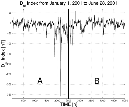
We expect that precisely the interplay between regularity / irregularity and amplitude characteristics should be learnt by ANNs to achieve superior performance. The simplest way to realize that is to add, besides the amplitudes of the analysed variables, the corresponding series of Hölder exponents to the ANN input. The following ACE SW parameters with hour time resolution were used: , , , , , . The time evolution of 1 hour index from January 1 to July 28, 2001 was considered. The time series of SW parameters were preprocessed using principal component () analysis [Gnanadesikan(1977), Reyment and Jöreskog(1996)]. The linear combinations of normalized SW parameters, their derivatives and combinations: , , , , , , , , , , , , , , , were used for the calculation of the ’s. It was shown by [Jankovičová et al.(2002)], that for the considered set of SW parameters, most of the variance of SW fluctuations is controlled by the first two components. In this paper we use and as SW input time series.
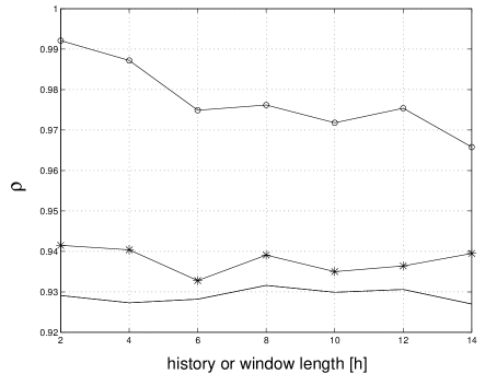
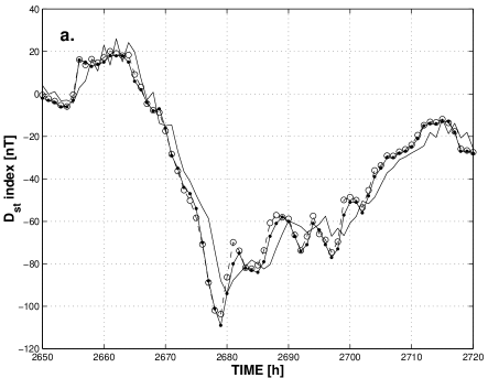
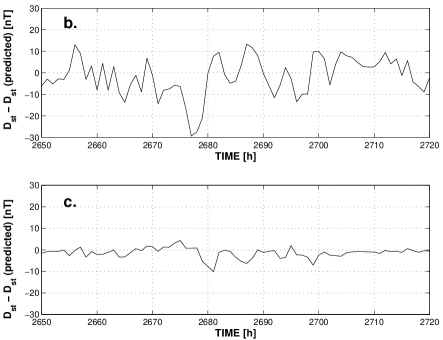
The local scaling characteristics of the principal components are described in the same way as of the other SW parameters. The time interval under study was divided into two subsets. The first one (part A in Figure 5) from January 1 to March 14, 2001 was used for ANN training while the second one (part B in Figure 5) from March 15 to July 28, 2001 represented independent set for prediction, not included in ANN training process. The influence of inclusion of local Hölder exponents on ANN performance was tested for a set of values of history and window length , whilst . In all cases analysed here a feedback consisting of past values of index was set. Figure 6 shows the dependence of correlation coefficient (Equation 6) in three different cases: 1.) Hölder exponents are not considered on input at all - only , and the feedback with history (indicated by a continuous line); 2.) Hölder exponents of and vectors are added as input (marked by ””); 3.) as in case 2.), but Hölder exponents describing the local scaling properties of past values are also added as an extra input (depicted by ”o”). The effect of the inclusion of Hölder exponents is evident mainly in the superior performance of ANNs in case 3. The correlation coeficient achieves its maximum at h and decreases with increasing and . At the same time ANN performance is practically unchanged in cases 1 and 2 when and increase. We mention that without the feedback slowly increases with [Jankovičová et al.(2002)]. As it can be seen, the consideration of scaling properties of and SW data enhances a little the performance level of ANN, but a real improvement is achieved when the singularity or regularity properties of geomagnetic fluctuations are taken into account, too (case 3). It seems to confirm our expectation that the information on local scaling properies of signals put to the input layer allows to learn input-output relations better accounting for changing activity levels more effectively. The analysis of (Equation 5) leads to the same conclusion. For demonstration 1 hour ahead predictions of an intense geomagnetic storm are shown in Figure 7a. Two methods are compared (Figure 7b, c): case 1 as defined above, when the index is predicted without Hölder exponents and case 3, with the information on ’s (, and ) added to the input layer (the cases 1 and 2 are similar). Easy to recognize that the method using ’s (case 3) allows to predict almost all the variance in the data with and nT having h. At the same time , nT for h (Figure 6 in case without Hölder exponents). In comparison, [Wu and Lundstedt(1996)] have exploited Elman recurrent ANNs to predict the index 1 hour ahead only from SW data. They achieved and nT.
4 Conclusions
We presented a prediction technique which uses the extra information on local scaling exponents to improve the performance of a layered ANN with feedback.
It was demonstrated that the Hölder exponents are time
dependent and change from point to point exhibiting large deviations from
the mean value , mainly during enhanced activity levels
of fluctuations. A peculiar interplay between regularity / irregularity features
(described by ) and amplitude characteristics of disturbances was
found and demonstrated on examples of SW and geomagnetic data. ANN performance was
significantly improved by putting the Hölder exponent time series of
corresponding SW and geomagnetic past data to the input layer yielding
the least error of 2 nT for short history h and window
length h. The results obtained without
Hölder exponents were the worst
( nT). Only a small improvement if any was achieved
when the Hölder exponents of SW and were added
only ( nT).
It means that to understand and model better
the magnetospheric response, in addition to SW input and geomagnetic history
(feedback), the scaling and irregularity / regularity features of magnetospheric
fluctuations should also be taken into account. It is not an
unexpected result,
however, because recent nonlinear theories on SWMC or magnetotail dynamics involve
or predict the appearance of scalings, irregularities (singularities)
and turbulence [Galeev et al.(1986), Chang(1999), Chapman et al.(1999), Klimas et al.(2000)].
To fully exploit this approach on experimental basis, further investigations of
scalings and singularity features of fluctuations in different inner and outer
regions of the magnetosphere will be necessary.
Acknowledgements
The authors wish to acknowledge valuable discussions with P. Kovács,
D. Vassiliadis and N. Watkins. index
from WDC Kyoto are gratefully acknowledged.
We are grateful to N. Ness (Bartol Research Institute) and D.J. McComas
(Los Alamos National Laboratory) for making the ACE data available.
This work was supported by VEGA grant 2/6040.
References
- [Antoni et al.(2001)] Antoni, V., Carbone, V., Cavazzana, R., Regnoli, G., Vianello, N., Spada, E., Fattorini, L., Martines, E., Serianni, G., Spolaore, M., Tramontin, L., and Veltri, P., Transport processes in reversed-field-pinch plasmas: inconsistency with the self-organized criticality paradigm, Phys. Rev. Lett., 87, 045001-1-045001-4, 2001.
- [Bargatze et al.(1985)] Bargatze, L.F., Baker, D.N., McPherron R.L. and Hones, E.W., Magnetospheric response to the IMF: substroms, J. Geophys. Res., 90, 6387, 1985.
- [Blanchard and McPherron(1994)] Blanchard, G.T. and McPherron, R.L., A bimodal response function relating the solar wind electric field to the AL index, in Artificial Intelligence Applications in Solar Terrestrial Physics, Joselyn, J., Lundstedt, H., Trolinger, j., editors, 153–158, Boulder, NOAA, 1994.
- [Borovsky et al.(1997)] Borovsky, J. E., Elphic, R. C., Funsten, H. O., and Thomsen, M. F., The Earth’s plasma sheet as a laboratory for flow turbulence in high-beta MHD, J. Plasma Phys., 57, 1–34, 1997.
- [Bruno et al.(1999)] Bruno, R., Bavassano, B., Pietropaolo, E., Carbone, V., and Veltri, P., Effects of intermittency on interplanetary velocity and magnetic field fluctuations anisotropy, Geophys. Res. Lett., 26, 3185–3188, 1999.
- [Burlaga(1991)] Burlaga, L. F., Intermittent turbulence in the solar wind, J. Geophys. Res, 96, 5847–5851, 1991.
- [Carbone(1994)] Carbone, V., Scaling exponents of the velocity structure functions in the interplanetary medium, Ann. Geophys., 12, 585–590, 1994.
- [Chang(1999)] Chang, T., Self-organized criticality, multi-fractal spectra, sporadic localized reconnections and intermittent turbulence in the magnetotail, Phys. Plasmas, 6, 4137–4145, 1999.
- [Chapman et al.(1998)] Chapman, S. C., Watkins, N. W., Dendy, R. O., Helander, P., and G. Rowlands, A simple avalanche model as an analogue for magnetospheric activity, Geophys. Res. Lett., 25, 2397–2400, 1998.
- [Chapman et al.(1999)] Chapman, S. C., Dendy, R. O., and G. Rowlands, A sandpile model with dual scaling regimes for laboratory, space and astrophysical plasmas, Phys. Plasmas, 6, 4169, 1999.
- [Consolini et al.(1996)] Consolini, G., Marcucci, M. F., and Candidi, M., Multifractal structure of auroral electrojet index data, Phys. Rev. Lett., 76, 4082–4085, 1996.
- [Consolini and De Michelis(1998)] Consolini, G., and De Michelis, P., Non-Gaussian distribution function of AE-index fluctuations: Evidence for time intermittency, Geophys. Res. Lett., 25, 4087–4090, 1998.
- [Consolini and Lui(1999)] Consolini, G., and Lui, A. T. Y., Sign-singularity analysis of current disruption, Geophys. Res. Lett., 26, 1673–1676, 1999.
- [Freeman et al.(2000)] Freeman, M.P., Watkins, N.W., and Riley, D.J., Power law burst and inter-burst interval distributions in the solar wind: turbulence or dissipative SOC?, Phys. Rev. E, 62, 8794–8797, 2000.
- [Galeev et al.(1986)] Galeev, A. A., Kuznetsova, M. M., and Zeleny, L. M., Magnetopause stability threshold for patchy reconnection, Space Sci. Rev., 44, 1–41, 1986.
- [Gnanadesikan(1977)] Gnanadesikan, R., Methods for statistical data analysis of multivariate observations, John Wiley and Sons, Inc., New York, 1977.
- [Gonzalez and Tsurutani(1987)] Gonzalez, W.D., and Tsurutani, B.T., Criteria of interplanetary parameters causing intense magnetic storms ( -100 nT), Planet. Space Sci., 35, 1101–1109, 1987.
- [Guiheneuf et al.(1998)] Guiheneuf, B., Jaffard, S. and Véhel, J.L., Two results concerning Chirps and 2-microlocal exponents prescription, Appl. Comp. Harm. Anal., 5, 487–492, 1998.
- [Halsey et al.(1986)] Halsey, T.C., Kadanoff, J.M.H., Procaccia, L.P., and Shraiman, B.I., Fractal measures and their singularities: the characterization of strange sets, Phys. Rev. A, 33, 1141, 1986.
- [Hernandez et al.(1993)] Hernandez, J.V., Tajima, T., and Horton, W., Neural net forecasting for geomagnetic activity, Geophys. Res. Lett., 20, 23, 2707, 1993.
- [Iyemori et al.(1979)] Iyemori, T., Maeda, H. and Kamei, T., Impulse response of geomagnetic indices to interplanetary magnetic field, J. Geomagn. Geoelectr., 6, 577, 1979.
- [Jaffard and Meyer(1996)] Jaffard, S. and Meyer, Y., Wavelet methods for pointwise regularity and local oscillations of functions, Memoirs of the A.M.S., 123, 587, 1996.
- [Jankovičová et al.(2001)] Jankovičová, D., Dolinský, P., Valach, F. and Vörös, Z., Neural network based nonlinear determination of the AE index, Contr. Geophys. & Geodesy, 31, 343–346, 2001.
- [Jankovičová et al.(2002)] Jankovičová, D., Dolinský, P., Valach, F. and Vörös, Z., Neural network based nonlinear prediction of magnetic storms, J. Atmosph. Solar-Terr. Phys., 2002, in press.
- [Klimas et al.(2000)] Klimas, A. J., Valdivia, J. A., Vassiliadis, D., Baker, D. N., Hesse, and Takalo, J., Self-organized criticality in the substorm phenomenon and its relation to localized reconnection in the magnetospheric plasma sheet, J. Geophys. Res., 105, 18765–18780, 2000.
- [Kovács et al.(2001)] Kovács, P., Carbone, V., and Vörös, Z., Wavelet-based filtering of intermittent events from geomagnetic time series, Planet. Space Sci., 49, 1219–1231, 2001.
- [Kröse and Smagt(1996)] Kröse, B. and Smagt, P., An introduction to neural networks, The University of Amsterdam, 1996.
- [Mallat and Hwang(1992)] Mallat, S.G., and Hwang, W.L., Singularity detection and processing with wavelets. IEEE Trans. Inform. Theory, 38(2), 617–643, 1992.
- [Marsch et al.(1996)] Marsch, E., Tu, C. Y., and Rosenbauer, H., Multifractal scaling of the kinetic energy flux in solar wind turbulence, Ann. Geophys., 14, 259–269, 1996.
- [McPherron et al.(1988)] McPherron, R.L., Baker, D.N., Bargatze, L.F, Clauer, C.R. and Holzer, R.E., IMF control of geomagnetic activity, Adv. Space Res., 8, 71, 1988.
- [Munsami (2000)] Munsami, V., Determination of the effects of substorms on the storm-time ring current using neural networks, J. Geophys. Res. , 105, 27833–27840, 2000.
- [Muzy et al.(1994)] Muzy, J.F., Bacry, E. and Arneodo, A., Multifractal formalism revisited with wavelets, Int. J. Bifurc. Chaos, 4, 245–302, 1994.
- [Price et al.(1994)] Price, C.P., Prichard, D. and Bischoff, J.E., Non-linear input/output analysis of the auroral electrojet index, J. Geophys. Res., 99(7), 13277, 1994.
- [Riedi and Véhel(1997)] Riedi, R.H. and Véhel, J.L., Multifractal properties of TCP traffic:a numerical study, INRIA Res. Rep., 3129, 1997.
- [Reyment and Jöreskog(1996)] Reyment, R.A. and Jöreskog, K.G., Applied factor analysis in the natural sciences, Cambridge University Press, 1996.
- [Rumelhart et al.(1986)] Rumelhart, D.E., Hinton, G., and Williams, R., Learning representations by back-propagating errors, Nature, 323, 533, 1986.
- [Tu et al.(1996)] Tu, C. Y., Marsch, E., and Rosenbauer, H., An extended structure-function model and its application to the analysis of solar wind intermittency properties, Ann. Geophys., 14, 270–285, 1996.
- [Vassiliadis et al.(1995)] Vassiliadis, D., Klimas, A.J., Baker, D.N. and Roberts, D.A., A description of the solar wind-magnetosphere coupling based on nonlinear filters, J. Geophys. Res., 100, 3495–3512, 1995.
- [Véhel and Vojak(1998)] Véhel, J.L., and Vojak, R., Multifractal analysis of choquet capacities: preliminary results, Adv. Appl. Math., 20, 1–43, 1998.
- [Vörös(2000)] Vörös, Z., On multifractality of high-latitude geomagnetic fluctuations, Ann. Geophys., 18, 1273–1282, 2000.
- [Watkins et al.(2001)] Watkins, N. W., Freeman, M.P., Chapman, S. C. and Dendy, R.O., Testing the SOC hypothesis for the magnetosphere, J. Atmosph. Sol. Terr. Phys., 63, 1435–1445, 2001.
- [Weigel et al.(1999)] Weigel, R.S., Horton, W., Tajima, T. and Detman, T., Forecasting Auroral electrojet activity from solar wind input with neural networks, Geophys. Res. Lett., 26, 1353–1356, 1999.
- [Weigel(2000)] Weigel, R.S., Prediction and modeling of magnetospheric substorms, Thesis, 2000.
- [Wu and Lundstedt(1996)] Wu, J.G. and Lundstedt, H., Prediction of geomagnetic storms from solar wind data using Elman recurrent neural networks, Geophys. Res. Lett., 23, 319–322, 1996.