Energy controlled insertion of polar molecules in dense fluids

Abstract

We present a method to search low energy configurations of polar molecules in the complex potential energy surfaces associated with dense fluids. The search is done in the configurational space of the translational and rotational degrees of freedom of the molecule, combining steepest-descent and Newton-Raphson steps which embed information on the average sizes of the potential energy wells obtained from prior inspection of the liquid structure. We perform a molecular dynamics simulation of a liquid water shell which demonstrates that the method enables fast and energy-controlled water molecule insertion in aqueous environments. The algorithm finds low energy configurations of incoming water molecules around three orders of magnitude faster than direct random insertion. This method is an important step towards dynamic simulations of open systems and it may also prove useful for energy-biased ensemble average calculations of the chemical potential.

Many processes of physical, chemical and biological interest involve open systems which exchange matter with their surroundings. Molecular dynamics (MD) and Monte Carlo (MC) simulations of these systems often require a method for molecule insertion and, therefore, a method for searching configurations with prescribed (low) potential energy. Indeed, a randomly placed molecule is likely to overlap with pre-existing atoms, releasing into the system a very high amount of energy.

The most natural setting for these systems is the grand canonical (GC) ensemble. Several methods for GC simulations require the location of energy cavities for insertion (such as cavity-biased methods for GCMC Allen and Tildesley (1987); Adams (1975); Mezei (1987)) or careful control of the solvent insertion energy in the case of GCMD Jie Ji and Pettitt (1992); G.C. Lynch (2000). Mass, momentum and energy transfer are also a key feature of a class of hybrid methods for non-equilibrium simulations which couple an open MD region with an interfacing continuum-fluid-dynamics domain Delgado-Buscalioni and Coveney (2003a); Flekkøy et al. (2000). Open boundaries in such hybrid schemes can avoid finite size effects in small MD simulation boxes Barsky et al. (2004), thereby saving on computational time. These sort of open boundaries could also be used to improve the closed “water shells” widely used to hydrate restricted subdomains King and Warshel (1989) in many MD simulations of biological systems.

Water insertion is also particularly important in protein simulations. For instance, it is possible to study protein unfolding via gradual water insertion in the protein’s cavities Goodfellow et al. (1996); M.A.Williams et al. (1997). On the other hand, water molecules buried in protein cavities at very low energies are essential for protein structure and function Zhang and Hermans (1996); Hofacker and Schulten (1998); Jensen et al. (2003). Indeed, some tools for MD simulations (such as dowser Zhang and Hermans (1996)) are specialised for water insertion in hydrophilic cavities, leaving empty however the larger hydrophobic cavities which frequently contain stable yet disordered water molecules relevant to protein functionHofacker and Schulten (1998); Cai et al. (2003).

Several methods for the calculation of ensemble averages require sampling the potential energy released to the system upon insertion of a test molecule Allen and Tildesley (1987); Bennett (1976); K.S.Shing and K.E.Gubbins (1982); Lu et al. (2003). Examples include calculation of the chemical potential, hydration energies and pair distribution functions Guillot et al. (1991). The applicability of these methods can be expanded to dense fluids using techniques that bias the sampling towards low energy configurations. Some of these techniques, such as cavity-biased Jedlovszky and Mezei (2000); Pohorille and Wilson (1996) or excluded volume map G.L.Deitrick et al. (1989) sampling, are however hampered by the considerable amount of time needed to find “cavities” where the test molecule could be inserted without overlapping with others. In fact, these cavities are just proxies to search low energy configurations which could better be identified by an energy controlled insertion method.

The algorithms for water insertion proposed in the literature usually involve rather lengthy steps which comprise three separate parts: location of a suitable “cavity”, normally using an expensive grid search with $O(10^{6})$ different cells Mezei (1987); Pohorille and Wilson (1996); Jie Ji and Pettitt (1992); random insertion in the cavity, followed by a large number of energy minimisation steps (either of the inserted molecule Jie Ji and Pettitt (1992); Zhang and Hermans (1996) or of the entire system Goodfellow et al. (1996)) and, finally, thermostatting the whole system over a one to ten picoseconds period to extract the extra energy released upon insertion. In this article, we present a method to locate low energy configurations of dense liquids that allows insertion of solvent molecules on-the-fly: avoiding expensive grid search, non-local energy minimisation and thermostatting steps.

On the potential energy surface, low energies are located inside energy wells whose local minima span a relatively large range of energy values. The main idea of the present method is to reconstruct the energy landscape with a limited number of probes by constraining the search to be inside the energy wells. In fact, any excursion outside the explored well implies the loss of all the information accumulated on the current well which is effectively equivalent to a random restart. Efficiency is obtained by minimising both the number of probes needed to determine if the target energy is found within the well and the number of explored wells per successful insertion. The present minimisation algorithm generalises non-trivially to multiple degrees of freedom the usher algorithm for insertion of Lennard-Jones atoms Delgado-Buscalioni and Coveney (2003b). It shares with some other global minimisation methods the recipe of applying in turns random moves and local energy minimisation Levitt and Warshel (1975); Li and Scheraga (1987); Saunders (1987). However, it is distinguished from these others in the way the minimisation is performed via a combined steepest-descent and Newton-Raphson iterator which is tailored adaptively to the structure of the potential energy landscape being searched.

The method uses local information on the gradient and the average size of the potential wells, which are dependent on the molecule’s location and the thermodynamic state respectively. The input parameters specify the maximum distance $\Delta R$ and rotation angle $\Delta\Theta$ that the incoming molecule can jump without exiting the current well together with a measure of the roughness of the potential energy surface $\Delta E_{R}$. The insertion algorithm starts by selecting a random location for the centre of mass of the molecule and placing the atoms at the equilibrium bond and angle positions in a random orientation. The non-bonded potential energy of an incoming molecule is given by

$$U=\frac{1}{2}\sum_{i\neq j}V_{LJ}(r_{ij})+\frac{1}{2}\sum_{i\neq j}V_{C}(r_{ij}),$$ (1)

where $V_{LJ}$ and $V_{C}$ are the Lennard-Jones and Coulomb pair potentials respectively Allen and Tildesley (1987) and the index i runs over the atoms of the molecule and j over all other atoms, which remain fixed while inserting. The energy $E=2U$ released to the system upon insertion is computed and compared with the target energy $E_{T}$. The insertion succeeds once the energy difference $\Delta E=E-E_{T}$ is less than a certain prescribed tolerance set here at $10^{-3}$ Kcal/mol.

It is likely that for the random starting configuration $\Delta E$ will be a large positive value because there is a high chance that the inserted molecule will overlap with others. Then, the force ${\bf F}=\sum_{i}{\bf F}_{i}$ applied to the centre of mass ${\bf r}_{cm}$ and torque ${\bf\tau}=\sum_{i}{\bf r}_{cm,i}\times{\bf F}_{i}$ are used to compute the next displacement and rotation. Here, the index $i$ runs over the atoms of the inserted molecule and ${\bf r}_{cm,i}={\bf r}_{i}-{\bf r}_{cm}$. The molecule is translated by $\delta r=\min(\Delta E/F,\Delta R)$ where $F$ is the magnitude of the force on the centre of mass and $\Delta R$ is the maximum displacement. With the reference system fixed to the molecule, we then compute the rotation angle around the torque axis $\delta\theta=\min(\Delta E/\tau,\Delta\Theta)$ and rotate the molecule around the centre of mass. The resulting update rule is finally given by

$${\bf r}^{n+1}_{cm} = {\bf r}^{n}_{cm}+\frac{{\bf F^{n}}}{F^{n}}\delta r,$$

$${\bf r}^{n+1}_{cm,i} = {\cal R}_{{\bf\tau}^{n}}{\bf r}^{n}_{cm,i},$$ (2)

where ${\cal R}$ is the rotation matrix around the axis of torque of angle $\delta\theta$. This is equivalent to a first order steepest descent procedure for large energy differences and a second order Newton method for energy close to the target energy Delgado-Buscalioni and Coveney (2003b). The angular minimisation is stopped when the angle $\delta\theta$ is less than $1^{\circ}$ to avoid oscillations due to the coupling of rotational and translational degrees of freedom. If during the iterations $\Delta E$ increases by more than $\Delta E_{R}$ then the current attempt is abandoned and a new random configuration is generated. This provides a threshold to control the amount of time spent searching in the well and the number of wells explored.

The insertion algorithm in Eq. (2) does not require a baroque implementation and indeed can be easily included in any molecular dynamics program. The code used here is based on the serial version of a well established parallel molecular dynamics code NAMD with the Charmm27 force field Kalé et al. (1999), but it has been designed to interface easily with any other serial or parallel MD code. The search algorithm applies in general to small polar molecules but given its importance we focus on controlled insertion of water molecules in aqueous environments. We use the TIP3P model for water, widely utilised in biological simulations Jorgensen et al. (1983). This water model is based on three interaction sites, bonds (O-H) and angle (H-O-H) being constrained rigidly or, in its flexible version (used here), by a harmonic potential with equilibrium configurations of 0.96 Å and $104.52^{\circ}$ respectively.

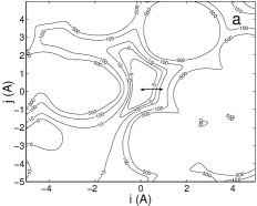
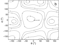
Figure 1: Contour plot of the potential energy landscape in Kcal/mol: (a) for translation relative to the axes i and j fixed to the water molecule; (b) for a rotation $\theta$ about the axis j and $\phi$ about the axis k for an equilibrated periodic liquid water system at 300K and density 0.96 $g/cm^{3}$. The maximum translational displacement $\Delta R=1.0$ Å and maximum rotational angles $\Delta\Theta=\Delta\Phi=45^{\circ}$ are indicated by double-headed arrows. For visual convenience angles smaller than $-90^{\circ}$ and larger than $90^{\circ}$ in $\theta$ are plotted although being redundant.

As stated, the restriction on the maximum displacement and rotation has the effect of limiting the search to the current potential well. For water, the maximum displacement can be extracted from the oxygen-hydrogen pair distribution function $g_{OH}$ Jorgensen et al. (1983). We found that an optimum value for the maximum displacement $\Delta R=1$ Å is half of the first peak in $g_{OH}$ which is around 2 Å. Exploring the potential energy landscape provides another simple way of obtaining the input parameters. In Fig. 1a, we show a cross-section of the potential energy surface for a displacement of up to 5 Å around an equilibrated water molecule in the direction of the axes ${\bf i}$ and ${\bf j}$. The unit vectors ${\bf i,j,k}$ form a reference system fixed rigidly to the water molecule with the axis ${\bf i}$ being in the direction of the dipole. As shown in Fig. 1a the optimum value of $\Delta R$ is approximately the radius of the potential energy well, corroborating information furnished from the pair distribution function. It is more difficult to obtain structural information for the angular degrees of freedom. However, a simple inspection of Fig. 1b provides a gross estimate of potential energy wells in the rotational degrees of freedom as being between $90-100^{\circ}$ wide; therefore the maximum rotation can be fixed at $\Delta\Theta=45^{\circ}$. The value of $\Delta E_{R}$, which sets the maximum uphill energy jump allowed in one move, is important to reduce the number of unsuccessful wells explored. We found that an optimal value is near $\Delta E_{R}=3$ Kcal/mol.

It is well known that the local structure of liquid water at equilibrium consists of a hydrogen bond network formed by oxygen and hydrogen atoms from neighbouring water molecules. This structure makes it very hard for an incoming water molecule to find low energy configurations by forming hydrogen bonds with pre-existing molecules. However, the insertion algorithm needs only to control the thermodynamics by inputting into the system a specified amount of energy which depends on the ensemble considered. We performed an MD simulation of bulk water using a simple spherical water shell to show that it is possible to insert water molecules on-the-fly while precisely controlling the energy released to the system. In a previous work Delgado-Buscalioni and Coveney (2003b) considering Lennard-Jones atoms, it was shown that this procedure ensures thermodynamic consistency after a relaxation time of the order of the collision time. We set up an equilibrated TIP3P bulk water system within a sphere of radius $37.5$ Å at 300K and a pressure of 1 atm. The simulations were run with a 12 Å cutoff radius and without corrections to the long ranged electrostatic forces Kalé et al. (1999). The water molecules in the outer shell of length $d=12.5$ Å play the role of a reservoir confined in the sphere by a simple constant radial force field specified by an acceleration ${\bf g}$ acting only within the outer shell. The effect of this force is a linear decay of the pressure in the water shell according to the usual formula for the hydrostatic pressure in an incompressible fluid $P_{1}=P_{0}-\rho gd$, where $P_{1}$ is the pressure at the surface of the water sphere and $P_{0}$ is the pressure of the bulk that we want to maintain. We impose $P_{1}=0$ by setting $g=P_{0}/(\rho d)$.

In the present set up, the flow rate of molecules to the inner shell is controlled by the applied pressure force, while the number of reservoir molecules in the outer shell is fixed at the bulk density. This implies that molecules which, due to fluctuations or sudden pressure waves, move outside the sphere are removed and reinserted using the insertion method at a random location in the outer shell, with a velocity given by the Maxwell-Boltzmann distribution at 300K. We note that the present setting can be generalised to avoid finite-size effects due to periodic boundary conditions in a hydrodynamically consistent wayDelgado-Buscalioni and Coveney (2003a). The total energy of the system can be fixed by setting the amount of energy released upon insertion equal to the energy lost when a molecule moves out through the open boundary Delgado-Buscalioni and Coveney (2003a). On average, the exchanged potential energy per molecule is equal to the mean energy per molecule: by inserting at this energy target we kept the total energy under control (without drift) with no thermostat at all. In other situations, such as at constant temperature, it is sufficient to release a moderately greater energy, for example equal to the excess chemical potential, which can be thermalized dynamically by the thermostat.

An estimate of the efficiency of this insertion method can be obtained by determining the average number of energy evaluations, including failed well searches, needed to insert a single water molecule at the specified energy. Each iteration of the insertion algorithm corresponds to one energy evaluation on the solvent molecule, which is a three atom-force calculation for TIP3P water. In particular, it takes an average of $206$ iterations, exploring $34$ wells, to insert at the reference energy of the mean energy per molecule ($-11$ Kcal/mol), and $36$ iterations (only $6$ wells) at the energy of the excess chemical potential (-5.8 Kcal/mol, calculated using the Bennett method Bennett (1976)). We note that the computational cost required by the insertion method in a typical MD simulation is quite small. For instance, in the simulation of the open water shell mentioned above, incoming water molecules were inserted at a target energy of $E_{T}=-11$Kcal/mol within a volume of $155.4$nm³ at a rate of $141$ per picosecond. The amount of CPU time devoted to insertion was only $3\%$ of the grand total of the simulation.

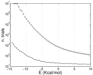
Figure 2: Number of energy evaluations per molecule required to insert a water molecule while releasing an energy less than E (Kcal/mol) to the system. The proposed insertion algorithm (crosses) is around three orders of magnitude faster than random insertion (circles) at low energies. The histogram for random insertion is computed from $10^{7}$ trials.

Interestingly, the mean number of iterations to explore a well which leads to the correct target energy is only around $12$, independent of the target energy. The method may be improved further by reducing the total number of searched wells but it is already optimal in the sense that the number of iterations to explore a single well does not depend on the target energy. Future applications may require searching many more degrees of freedom, e.g. conformational searches, for which it is impractical to fix each maximum displacement a priori. In this case, it would be useful to set up an adaptive rule to infer the input parameters from the efficacy of the search itself.

It is useful to compare our insertion algorithm with a direct random insertion. To this end, the probability distribution $f(E)$ of releasing a total energy $E$ upon random insertion was estimated by computing a histogram from $10^{7}$ random insertion trials. The number of trials required to obtain an energy smaller than E is given by the reciprocal of the cumulative distribution $1/F(E)$ where $F(E)=\int_{-\infty}^{E}f(E^{\prime})dE^{\prime}$. This number is compared with the number of iterations (energy evaluations) required by the insertion algorithm in Fig. (2). The insertion algorithm is around three orders of magnitude faster than a random insertion for energies lower than the chemical potential and so may provide an efficient alternative to biased methods, such as cavity-biased sampling Jedlovszky and Mezei (2000); Pohorille and Wilson (1996), to reconstruct the probability distribution $f(E)$. Indeed, the present algorithm enables one to identify the important low energy regions very accurately where an un-biased sampling can be performed. This appealing approach enables fast computation of the chemical potential from the probability distribution $f(E)$ at low energiesDelgado-Buscalioni et al. (2004).

In summary, we have reported a new method for the insertion of polar molecules in dense fluids by a generalisation of the usher protocol Delgado-Buscalioni and Coveney (2003b). The energy minimisation is applied concurrently to all degrees of freedom (translational and rotational for water) and is independent of the specific potential used. Indeed, the method is even more general. It may be applied to other problems related to conformational searches and minima of potential energy surfaces with many more degrees freedom. Given its importance for computational biology, we focused on water and demonstrated that it is possible to efficiently insert water molecules in aqueous environments while controlling the thermodynamic state. This task is commonly considered to be very time consuming, but we are able to achieve it at negligible computational cost thanks to a very efficient configurational search algorithm. The present algorithm is an essential tool for performing hybrid MD-continuum simulations Delgado-Buscalioni and Coveney (2003a); Barsky et al. (2004) of biological interest. Indeed, it represents an important step towards a general method for performing MD simulations of open systems, for which a dynamic calculation of the chemical potential Lu et al. (2003); Delgado-Buscalioni et al. (2004) could be used to control the insertion rate so as to maintain constant the solvent chemical potential.

This research was supported by the EPSRC Integrative Biology project GR/S72023 and by the EPSRC RealityGrid project GR/67699.

References

- Allen and Tildesley (1987) M. Allen and D. Tildesley, Computer Simulations of Liquids (Oxford University Press, 1987).
- Adams (1975) D. Adams, Mol. Phys. 29, 307 (1975).
- Mezei (1987) M. Mezei, Mol. Phys. 61, 565 (1987).
- Jie Ji and Pettitt (1992) T. C. Jie Ji and B. M. Pettitt, J. Chem. Phys. 96, 1333 (1992).
- G.C. Lynch (2000) B. G.C. Lynch, Chemical Physics 258, 405 (2000).
- Delgado-Buscalioni and Coveney (2003a) R. Delgado-Buscalioni and P. V. Coveney, Phys. Rev. E 67, 046704 (2003a).
- Flekkøy et al. (2000) E. G. Flekkøy, G. Wagner, and J. Feder, Europhys. Lett. 52, 271 (2000).
- Barsky et al. (2004) S. Barsky, R. Delgado-Buscalioni, and P. V. Coveney, J. Chem. Phys. 121, 2403 (2004).
- King and Warshel (1989) G. King and A. Warshel, J. Chem. Phys. 91, 3647 (1989).
- Goodfellow et al. (1996) J. M. Goodfellow, M. Knaggs, M. A. Williams, and J. M. Thornton, Faraday Discussions 103, 339 (1996).
- M.A.Williams et al. (1997) M.A.Williams, J.M.Thornton, and J.M.Goodfellow, Protein Engineering 10, 895 (1997).
- Zhang and Hermans (1996) L. Zhang and J. Hermans, Proteins:Struct. Func. Genet. 24, 433 (1996).
- Hofacker and Schulten (1998) I. Hofacker and K. Schulten, Proteins:Struct. Func. Genet. 30, 100 (1998).
- Jensen et al. (2003) M. Jensen, E. Tajkorshid, and K. Schulten, Biophysical Journal 85, 2884 (2003).
- Cai et al. (2003) S. Cai, S. Stevens, A. Budor, and E. Zuiderweg, Biochemistry 42, 9 (2003).
- Bennett (1976) C. H. Bennett, J. Comput. Phys. 22, 245 (1976).
- K.S.Shing and K.E.Gubbins (1982) K.S.Shing and K.E.Gubbins, Mol. Phys. 46, 1109 (1982).
- Lu et al. (2003) N. Lu, J. K. Singh, and D. A. Kofke, J. Chem. Phys. 118, 2977 (2003).
- Guillot et al. (1991) B. Guillot, Y. Guissani, and S. Bratos, J. Chem. Phys. 95, 3643 (1991).
- Jedlovszky and Mezei (2000) P. Jedlovszky and M. Mezei, J. Am. Chem. Soc. 122, 5125 (2000).
- Pohorille and Wilson (1996) A. Pohorille and M. A. Wilson, J. Chem. Phys. 104, 3760 (1996).
- G.L.Deitrick et al. (1989) G.L.Deitrick, L. Scriven, and H. Davis, J. Chem. Phys. 90, 2370 (1989).
- Delgado-Buscalioni and Coveney (2003b) R. Delgado-Buscalioni and P. V. Coveney, J. Chem. Phys. 119, 978 (2003b).
- Levitt and Warshel (1975) M. Levitt and A. Warshel, Nature 253, 694 (1975).
- Li and Scheraga (1987) Z. Li and H. A. Scheraga, Proc. Natl. Acad. Sci. USA 84, 6611 (1987).
- Saunders (1987) M. Saunders, J. Am. Chem. Soc. 109, 3150 (1987).
- Kalé et al. (1999) L. Kalé, R. Skeel, M. Bhandarkar, R. Brunner, A. Gursoy, N. Krawetz, J. Phillips, A. Shinozaki, K. Varadarajan, and K. Schulten, J. Comp. Phys. 151, 283 (1999).
- Jorgensen et al. (1983) W. L. Jorgensen, J. Chandrasekhar, and D. Madura, J. Chem. Phys. 79, 926 (1983).
- Delgado-Buscalioni et al. (2004) R. Delgado-Buscalioni, G. De Fabritiis, and P. Coveney, Fast calculation of the chemical potential using energy-biased sampling, preprint (2004).