Eigenmodes of index-modulated layers with lateral PMLs

Abstract

Maxwell equations are solved in a layer comprising a finite number of homogeneous isotropic dielectric regions ended by anisotropic perfectly matched layers (PMLs). The boundary-value problem is solved and the dispersion relation inside the PML is derived. The general expression of the eigenvalues equation for an arbitrary number of regions in each layer is obtained, and both polarization modes are considered. The modal functions of a single layer ended by PMLs are found, and their orthogonality relation is derived. The present method is useful to simulate scattering problems from dielectric objects as well as propagation in planar slab waveguides. Its potential to deal with more complex problems such as the scattering from an object with arbitrary cross section in open space using the multilayer modal method is briefly discussed.

1 Introduction

The perfectly matched layer (PML) is a fictitious material which does not reflect incident propagating waves regardless of the incident angle, frequency and polarization. It was firstly introduced by Berenger [1, 2] as a useful absorbing boundary condition to truncate the computational domain in finite-difference time-domain applications. A different formulation of the PML, given by Sacks et al. [3], is based on exploiting constitutive characteristics of anisotropic materials to provide a reflectionless interface. This formulation offers the special advantage that it does not require modification of Maxwell equations [3]. Both formulations of the PML are very popular among the electrical engineering community and their use in the optics community has been growing in the last few years [4]-[8]. PMLs look attractive, mainly because of their potential capacity to simulate open-structure problems by bounded computational domains, which consequently reduce significantly the computational costs involved in the calculations [9]-[11]. Even though this kind of medium is usually used in the framework of finite-element methods [12]-[14], there are also studies which incorporate the anisotropic absorber in different approaches [7], [15]-[19]. In particular, the modal approach appears as an interesting alternative for the description of the fields in index-modulated structures since it highlights the physics of the problem.

The modal approach has been applied by many authors to dielectric lamellar gratings in classical [20]-[22] as well as in conical mounting [23, 24]. In his work, Li [24] derived rigorously the eigenfunctions and also their completeness and ortogonality relations from the boundary-value problem. Later on, this formalism was extended to deal with multiply grooved lamellar gratings [25], where the eigenvalues equation for an arbitrary number of different dielectric zones was obtained and carefully analyzed for real and complex refraction indices. The modal formulation presented in [25] was then extended to deal with finite structures such as index-modulated apertures [26].

A further step on the development of the modal method was the application of the multilayer approximation [21] not only to infinite gratings [27] but also to finite structures with arbitrary shapes of the corrugations [28]-[30]. However, all these works were restricted to structures laterally closed by perfect conductors. If illuminated by finite beams, these structures can approximately simulate the scattering from purely dielectric finite structures [26], [28]-[30].

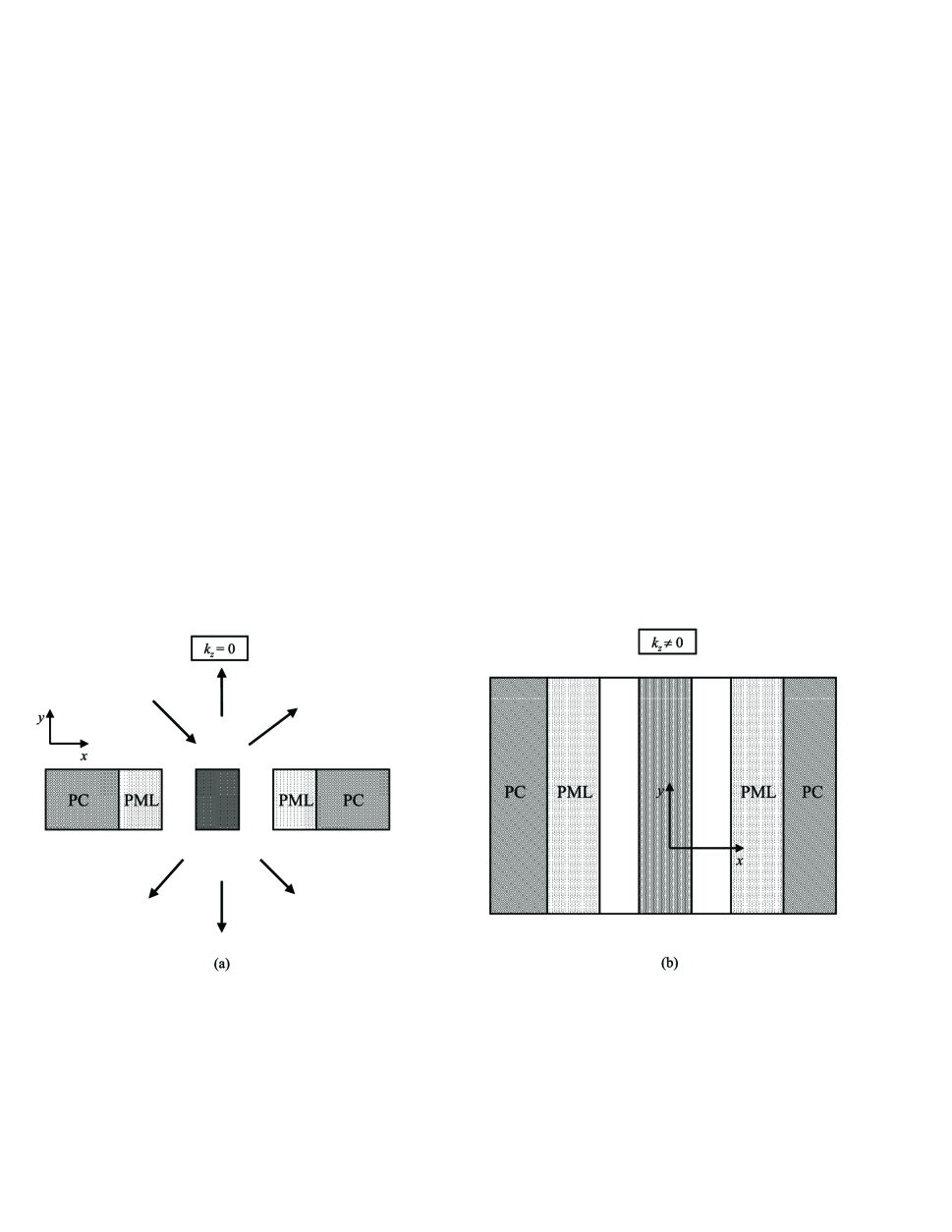
Figure 1: (a) Scheme of the scattering problem by an index-modulated aperture; (b) Scheme of the propagation problem in a planar slab waveguide.

It is well known that either the pseudeperiodic condition in infinite gratings or the assumption of perfect conductivity in finite structures forces the eigenvalues set to be discrete. On the other hand, open problems like propagation in dielectric waveguides or scattering from dielectric objects in open space, have a continuum set of eigenvalues. Therefore, it is allways convenient to limit the problem domain, in order to avoid large volumes of calculus. This can be done by means of perfectly matched layers, which ensure absorption and attenuation of the incident radiation and consequently simulate the open space better. A detailed formulation of the discretization of the continuous spectrum by means of a Dirichlet boundary condition for the complex plane has been recently presented [31], where the solution of the Sturm-Liouville problem for a layered structure is based on the PML boundary condition. The completeness of the eigenmodes of parallel plate waveguides with PML terminations has also been proven [32].

The purpose of this paper is to find the analytical expressions of the eigenmodes of a single index-modulated layer ended by PMLs at both sides, and also to derive the orthogonality relations that satisfy the set of eigenfunctions. A modal formulation is presented to apply the eigenmodes expressions to the solution of the scattering problem by a two-dimensional object of rectangular cross section in open space. We cover simultaneously the eigenmodes of an index-modulated aperture (schematized in Fig. 1a) as well as those of a planar slab waveguide (Fig. 1b), since both problems have an equivalent formulation. Numerical examples comparing the resulting eigenvalues with those found by a different approach [17] are shown. The present paper is more general than Ref. [17] since we find the eigenvalues and the eigenmodes of a layer comprising an arbitrary number of different homogeneous regions, with the aim of extending the modal method to more general structures ended by PMLs.

Finally, a brief discussion on the potential applicability of the modal method to the scattering problem by a 2-D object of arbitrary cross section in open space is given. This extension can be made by means of the multilayer approximation [21], and the application of any propagation algorithm such as the R-matrix [6, 7, 27][33]-[35].

2 Modal formulation

In this section we develop a rigorous method to find the exact modes of a structure as that of Fig. 2. The modes of such a structure can be then used to find the solution of waveguide problems and scattering problems.

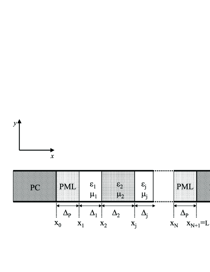
Figure 2: Configuration of the problem.

Consider an index-modulated layer invariant in the $\hat{z}$ direction, as shown in Fig. 2. Each homogeneous zone $x_{j}\leq x\leq x_{j}+\Delta_{j}$ of width $\Delta_{j}$ has a permittivity $\epsilon_{j}$ and a permeability $\mu_{j}$, where $\epsilon_{j}$ and $\mu_{j}$ can be complex numbers. The layer is ended at both sides by perfectly matched layers backed by perfect conductors. The PML is a particular anisotropic medium especially designed to absorb the received radiation [3], and its constitutive parameters are $\tilde{\epsilon}_{{\rm PML}}=\epsilon\tilde{\Lambda}$ and $\tilde{\mu}_{{\rm PML}}=\mu\tilde{\Lambda}$ where $\epsilon$ and $\mu$ are the permittivity and permeability of the adjacent isotropic zone, respectively. For an interface parallel to the $(y,z)$-plane, the tensor $\tilde{\Lambda}$ must be defined as:

$$\tilde{\Lambda}=\left[\begin{array}[]{ccc}1/b&0&0\\ 0&b&0\\ 0&0&b\end{array}\right]\;\;.$$ (1)

The parameter $b$ is a complex number: its real part is related to the wavelength inside the PML, and the imaginary part accounts for the losses in the material, i.e., the attenuation of the propagating waves.

As stated above, to find the eigenmodes of the structure depicted in Fig. 2 can be useful for waveguide and scattering problems. We are interested in studying the propagation of plane waves along the structure, and then a time dependence $e^{-i\omega t}$ ($\omega$ being the frequency of the plane wave) is implied and suppressed in all the paper. Since the structure is invariant in the $z$-direction, the problem can be separated into two scalar problems for $E_{z}$ (TM polarization) and $H_{z}$ (TE polarization). Then, the $x$- and $y$- components of the fields can be written in terms of the $z$-components [36].

Within the PML, Maxwell curl equations are

$$\vec{\nabla}\times\vec{E}=i\,\frac{\omega}{c}\,\mu\,\tilde{\Lambda}\,\vec{H}\;\;,$$ (2)

$$\vec{\nabla}\times\vec{H}=-i\,\frac{\omega}{c}\,\epsilon\,\tilde{\Lambda}\,\vec{E}\;\;,$$ (3)

where $c$ is the speed of light in vacuum and $\vec{E}$ and $\vec{H}$ are the electric and magnetic fields, respectively. In the case of a slab waveguide (Fig. 1b), we are interested in finding the solutions of Maxwell equations that have a $z$-dependence of the form $e^{ik_{z}z}$. Then, combining eqs. (2) and (3), and taking into account the invariance of the problem along the $\hat{z}$ direction, we get the propagation equations for a layer with $x$-dependent constitutive parameters, for both polarization modes:

$$\frac{\mu(x)}{b(x)}\frac{\partial}{\partial x}\left[\frac{1}{b(x)\mu(x)}\frac{\partial E_{z}(x,y)}{\partial x}\right]+\frac{\partial^{2}E_{z}(x,y)}{\partial y^{2}}+\gamma^{2}(x)E_{z}(x,y)=0\;\;,$$ (4)

$$\frac{\epsilon(x)}{b(x)}\frac{\partial}{\partial x}\left[\frac{1}{b(x)\epsilon(x)}\frac{\partial H_{z}(x,y)}{\partial x}\right]+\frac{\partial^{2}H_{z}(x,y)}{\partial y^{2}}+\gamma^{2}(x)H_{z}(x,y)=0\;\;,$$ (5)

where

$$\gamma^{2}(x)=\frac{\omega^{2}}{c^{2}}\epsilon(x)\mu(x)-k_{z}^{2}\;\;,$$ (6)

and $b(x)=1$ in the isotropic regions. For the scattering problem of a plane wave with wave vector $\vec{k}$ in the ($x,y$)-plane impinging on the structure (Fig. 1a), $k_{z}=0$ and then $\gamma^{2}(x)=k^{2}(x)=(\omega^{2}/c^{2})\epsilon(x)\mu(x)$. On the other hand, for a slab waveguide the problem is invariant in the $\hat{y}$ direction, and then $\partial_{y}=0$. Since the form of eqs. (4) and (5) is identical, we unify the treatment of both polarizations in a single differential equation

$$\frac{\sigma(x)}{b(x)}\frac{\partial}{\partial x}\left[\frac{1}{b(x)\sigma(x)}\frac{\partial\psi(x,y)}{\partial x}\right]+\frac{\partial^{2}\psi(x,y)}{\partial y^{2}}+\gamma^{2}(x)\psi(x,y)=0\;\;,$$ (7)

where

$$\sigma(x)=\left\{\begin{array}[]{ll}\mu(x)&\mbox{for TM polarization}\\ \\ \epsilon(x)&\mbox{for TE polarization}\end{array}\right.\;\;,$$ (8)

and $\psi$ represents either $E_{z}$ (TM case) or $H_{z}$ (TE case).

The eigenmodes of the structure are the set of linearly independent functions that satisfy by themselves the boundary conditions at all the interfaces $x=x_{j}$, $j=0,...,N+1$, and form a complete basis. In particular, since the layer is ended by a perfect conductor, we require that the tangential component of the electric field vanishes at $x=x_{0}$ and at $x=L$. To do so, we first solve eq. (7) in each region (isotropic and anisotropic) and then match these partial solutions correspondingly. For the most general case in which $\partial_{y}\neq 0$ a separated solution is proposed:

$$\psi(x,y)=X(x).Y(y)\;\;,$$ (9)

and substituting eq. (9) in eq. (7) we get two ordinary differential equations for the functions $X(x)$ and $Y(y)$

$$\frac{d^{2}Y}{dy^{2}}+v^{2}Y = 0\;\;,$$ (10)

$$\frac{\sigma(x)}{b(x)}\frac{d}{dx}\left[\frac{1}{b(x)\sigma(x)}\frac{dX}{dx}\right]+(\gamma^{2}(x)-v^{2})X = 0\;\;,$$ (11)

where $v$ is a constant. The formal solution of eq. (10) is straightforward:

$$Y(y)=a\cos(vy)+b\sin(vy)\;\;,$$ (12)

and we will now focus on the differential equation for $X(x)$. Notice that for the scattering problem $\gamma^{2}(x)=k^{2}(x)-v^{2}$ and for the slab waveguide problem $\gamma^{2}(x)=k^{2}(x)-k_{z}^{2}$. Then, we can unify both cases by setting $\rho=v^{2}$ in the first case and $\rho=k_{z}^{2}$ in the second case.

Eq. (11) together with the boundary conditions at the ends of the layer ($x=x_{0}$ and $x=L$) pose a boundary-value problem

$${\cal L}X=\rho X\;\;,$$ (13)

where $\cal L$ is the differential operator

$${\cal L}=\frac{\sigma(x)}{b(x)}\frac{d}{dx}\left[\frac{1}{b(x)\sigma(x)}\frac{d}{dx}\right]+\frac{\omega^{2}}{c^{2}}\mu(x)\epsilon(x)\;\;.$$ (14)

Since $b$ is a complex number, the operator $\cal L$ is a non-self-adjoint operator [37]. From the theory of non self-adjoint problems we know that the eigenvalues are infinite and complex in general, and the eigenfunctions do not necessarily form a complete and orthogonal set [37]. To find a useful solution to our problem, is then necessary to consider the adjoint problem of (13)

$${\cal L}^{*}X^{\dagger}=\rho^{\dagger}X^{\dagger}\;\;,$$ (15)

where the asterisk denotes complex conjugate and the ^† denotes adjoint. The eigenvalues of the adjoint problem are the complex conjugates of those of the direct problem, i.e.,

$$\rho^{\dagger}=\rho^{*}\;\;,$$ (16)

and the sets of eigenfunctions {$X_{m}(x)$} and {$X_{n}^{\dagger}(x)$} form a bi-orthonormal set such that $(X_{m},X_{n}^{\dagger})=\delta_{mn}$, where the internal product $(X_{m},X_{n}^{\dagger})$ is defined as

$$(X_{m},X_{n}^{\dagger})=\int\frac{b(x)}{\sigma(x)}X_{m}(x)(X_{n}^{\dagger}(x))^{*}dx\;\;.$$ (17)

Then, any continuous and piecewise differentiable function that satisfies the boundary conditions at the ends of the layer can be expanded as

$$f(x)=\sum_{m}A_{m}X_{m}(x)\;\;.$$ (18)

Taking into account these facts, we are going to find the solutions of eq. (11). In each homogeneous region ($j$), we propose a solution of the form

$$X_{j}(x)=A_{j}\cos[u_{j}(x-x_{j})]+B_{j}\sin[u_{j}(x-x_{j})]\quad\mbox{for $x_{j}\,<\,x\,<\,x_{j}+\Delta_{j}$}\;\;,$$ (19)

and substitute it into eq. (11) to get the dispersion relation

$$\frac{u_{j}^{2}}{b_{j}^{2}}+\rho=\gamma_{j}^{2}\;\;,$$ (20)

for the two kinds of zones we have in the structure: isotropic ($b_{j}=1$) and anisotropic ($b_{j}\in C$, $b_{j}\neq 1$). Notice that $\rho$ is a constant for each eigenmode, and the constitutive parameters of the PML satisfy $\tilde{\epsilon}_{0}=\epsilon_{1}\tilde{\Lambda}$, $\tilde{\mu}_{0}=\mu_{1}\tilde{\Lambda}$, and then $k_{0}^{2}=k_{1}^{2}$. The same occurs at the other end of the layer, and therefore, $u_{0}=b\,u_{1}$ and $u_{N}=b\,u_{N-1}$, i.e., the eigenvalue in the PML region is $b$ times the eigenvalue in the adjacent isotropic region. Then, the solution of eq. (11) in the whole layer can be expressed in terms of harmonic functions, where the amplitudes are such that satisfy the boundary conditions at the vertical interfaces, and the eigenvalues $u$ and $\rho$ satisfy the corresponding dispersion relation, depending on the zone (eq. (20)). Defining $\tilde{X}(x)$ as:

$$\tilde{X}(x)=\frac{u_{j}}{\sigma_{j}}\;[-B_{j}\cos{[u_{j}(x-x_{j})]}+A_{j}\sin{[u_{j}(x-x_{j})]}]\;\;\;\mbox{for $x_{j}\,<\,x\,<\,x_{j}+\Delta_{j}$}\;\;,$$ (21)

it is easy to verify that [26]:

$$X(x) = X(x_{j})\;\cos(u_{j}(x-x_{j}))-\frac{\sigma_{j}}{u_{j}}\tilde{X}(x_{j})\;\sin(u_{j}(x-x_{j}))\;,\;\;\;\mbox{for $x_{j}\,<\,x\,<\,x_{j}+\Delta_{j}$}$$

$$\tilde{X}(x) = \tilde{X}(x_{j})\;\cos(u_{j}(x-x_{j}))+\frac{u_{j}}{\sigma_{j}}X(x_{j})\;\sin(u_{j}(x-x_{j}))\;,\;\;\;\mbox{for $x_{j}\,<\,x\,<\,x_{j}+\Delta_{j}$}\;.$$ (22)

Notice that $\tilde{X}(x)$ is proportional to the normal derivative of $X(x)$ at the vertical interfaces, which implies that it represents the tangential component of the magnetic (electric) field in the case of TM (TE) polarization.

Equations (22) provide us with a relation between two field quantities at both sides of each homogeneous zone bounded by the interfaces at $x=x_{j}$ and $x=x_{j}+\Delta_{j}$. This relation can be expressed in matrix form as:

$$\left(\begin{array}[]{cc}{\bf X}(x_{j+1})\\ \\ \tilde{\bf X}(x_{j+1})\end{array}\right)={\bf M}_{j}(\rho)\left(\begin{array}[]{cc}{\bf X}(x_{j})\\ \\ \tilde{\bf X}(x_{j})\end{array}\right)\;\;,$$ (23)

where ${\bf M}_{j}(\rho)$ is a matrix given by:

$${\bf M}_{j}(\rho)=\left[\begin{array}[]{cc}\cos(u_{j}\Delta x_{j})&-\sin(u_{j}\Delta x_{j})\,\sigma_{j}/u_{j}\\ &\\ \sin(u_{j}\Delta x_{j})\;u_{j}/\sigma_{j}&\cos(u_{j}\Delta x_{j})\end{array}\right]\;\;.$$ (24)

${\bf X}(x)$ and $\tilde{\bf X}(x)$ represent vectors containing the modal functions $X_{m}(x)$ and $\tilde{X}_{m}(x)$, respectively, and $u$ and $\rho$ are related by the dispersion relation. The subscript $m$ denoting the mode has been suppressed as it is understood that relations (22)-(24) hold for each one of the modal terms. This procedure can be applied N times to get a relation between the fields at the perfectly conducting walls at $x=x_{0}$ and $x=x_{L}$. In such a case we have a relation of the form:

$$\left(\begin{array}[]{cc}{\bf X}(x_{L})\\ \\ \tilde{\bf X}(x_{L})\end{array}\right)=\tilde{\bf M}(\rho)\left(\begin{array}[]{cc}{\bf X}(x_{0})\\ \\ \tilde{\bf X}(x_{0})\end{array}\right)\;\;,$$ (25)

where $\tilde{\bf M}(\rho)$ is a product matrix:

$$\tilde{\bf M}(\rho)={\bf M}_{L}(\rho)\;{\bf M}_{L-1}(\rho)\;\ldots\;{\bf M}_{2}(\rho)\;{\bf M}_{1}(\rho)\;\;.$$ (26)

$\tilde{\bf M}(\rho)$ is a $2\times 2$ block matrix. This is a well known result from the theory of stratified media [38].

Imposition of the boundary condition at $x_{0}$ and at $x_{L}$, i.e., the tangential component of the electric field must vanish on the surface, yields a condition on the non-diagonal block elements:

$$\tilde{\bf M}_{12}(\rho) = 0\;\;\;\;\;\mbox{for TM polarization}$$ (27)

$$\tilde{\bf M}_{21}(\rho) = 0\;\;\;\;\;\mbox{for TE polarization}\;\;.$$ (28)

These conditions determine eigenvalues equations for $\rho$, that must be solved by means of numerical techniques. These equations have already been studied for structures formed by isotropic regions in the case of an infinite periodic grating [25] and of an index-modulated aperture [26, 29]. The expressions of the equations found in this work reduce to those in Refs. [26, 29] for $b=1$. Also, a recursive formula to find the eigenvalues equation of a layer with N different regions could be derived in the present case [29]. Finally, the eigenmodes of the layer bounded by perfectly matched layers backed by perfectly conducting walls are given by

$$X_{m}(x)=A_{mj}\cos[u_{mj}(x-x_{j})]+B_{mj}\sin[u_{mj}(x-x_{j})]\;\;\;\mbox{for $x_{j}\,<\,x\,<\,x_{j}+\Delta_{j}$}\;\;,$$ (29)

where $u_{mj}$ satisfy the corresponding eigenvalues equation (27) or (28). The modal coefficients $A_{mj}$ and $B_{mj}$ are easily obtained by successive application of eqs. (22)

$$A_{mj} = A_{m,j-1}\cos[u_{m,j-1}(x_{j}-x_{j-1})]+B_{m,j-1}\sin[u_{m,j-1}(x_{j}-x_{j-1})]$$

$$B_{mj} = \frac{u_{m,j-1}}{u_{mj}}\frac{\sigma_{j}}{\sigma_{j-1}}\left\{B_{m,j-1}\cos[u_{m,j-1}(x_{j}-x_{j-1})]-A_{m,j-1}\sin[u_{m,j-1}(x_{j}-x_{j-1})]\right\}\;\;.$$ (30)

3 Examples

The eigenvalues equation is the critical part of any modal formulation, particularly for layers comprising different kinds of materials. Equations of this kind have been solved in Refs. [25], [26] and [28] for real refractive indices (non lossy dielectrics) and in [30] for lossy materials. A detailed study of the respective equations has been performed in the above works to avoid numerical problems with the rootfinding algorithms. In [26],[28] and [29] the authors use the separation constant along the $y$ direction ($v^{2}$) as the variable of the equation, whereas for highly conducting metals, i.e. regions of refraction index with a large imaginary part, it is convenient to use the separation constant in the $x$ direction ($u$) as the variable [30]. This behaviour can be understood taking into account the location of the eigenvalues in two limit cases: (i) ideal dielectric isotropic material (real refraction index), and (ii) perfect conductor (infinite refraction index). In the first case, the eigenvalues ($v^{2}$) are real, and then, for small perturbations of the refraction index (lossy dielectrics) a small departure from these values is expected. On the contrary, for the perfect conductor the eigenvalues ($u$) are real and can be calculated analytically [39]. Therefore, we expect the eigenvalues corresponding to a highly conducting metal not to depart too much from those real values.

As a first example, we consider the case of a symmetric structure formed by three zones (PML - dielectric - PML) of widths $\Delta_{P}$ and $\Delta_{1}$, and then $u_{0}=u_{2}=u_{P}$. This example actually simulates the open space, and can be useful to study the coupling between a slab waveguide and open space [17]. For this case, the direct application of the procedure described in the previous section yields an eigenvalues equation for both polarization modes, that after some manipulation can be reduced to:

$$\sin(2u_{P}\Delta_{P}+u_{1}\Delta_{1})=0\;\;.$$ (31)

Taking into account that $u_{P}=u_{1}b$, the solutions of eq. (31) are

$$u_{1m}=\frac{m\pi}{2\,b\,\Delta_{P}+\Delta_{1}}\;\;,\;\;\;\mbox{for $m$ integer}.$$ (32)

The eigenvalues obtained in (32) are the same as those found by Derudder et al. by means of a coordinates transformation in the propagation equation (eqs. (16) and (17) in Ref. [17]).

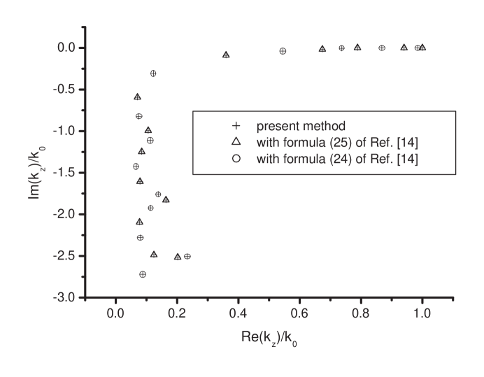
Figure 3: Comparison of the eigenvalues obtained by the present method and that of Derudder et. al (eqs. (24) and (25) in Ref. [17]) for a structure with 5 zones: $\Delta_{P}/\lambda=0.04$, $\Delta_{1}/\lambda=\Delta_{3}/\lambda=0.5$, $\Delta_{2}/\lambda=2$, $n_{1}=n_{3}=1$, $n_{2}=1.3$, $b=2-2i$, TM polarization.

It is important to remark that an increase in the number of homogeneous regions in the layer produces a more complex eigenvalues equation, since it is obtained from the determinant of a matrix product (eq. (26)). The number of terms and the number of trigonometric factors in each term increases, causing abrupt oscillations in the equation. However, since we are focusing on the solution of scattering problems from homogeneous objects in open space, the number of different regions to be considered in this case, including the PML, is restricted to five. The explicit expressions of the eigenvalues equations for five zones and for $\Delta_{1}=\Delta_{3}$ and $\mu_{j}=\mu_{0}\forall j$ are given in the Appendix for TE and TM polarizations. As it can be observed in Fig. 3 for TM polarization, the solutions of the equation are coincident with those obtained from eqs. (24) and (25) in Ref. [17]. These equations correspond to the eigenvalues equations for odd and even modes, respectively.

In Fig. 4 we show the evolution of the eigenvalues as the imaginary part of the PML parameter $b$ is increased, for a structure comprising five zones and TE polarization. For $Im(b)=0$, the eigenvalues $u_{1}$ are real, and their values depart from the real axis as $Im(b)$ is increased.

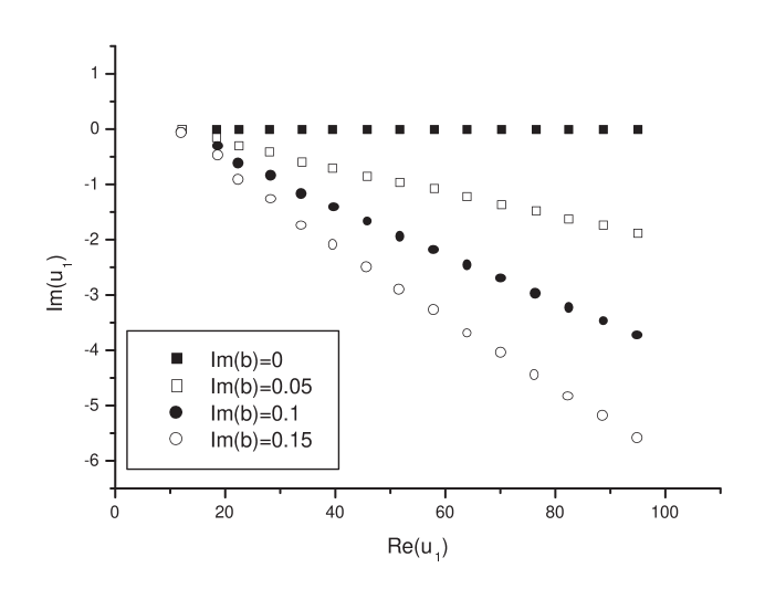
Figure 4: Evolution of the eigenvalues with the imaginary part of the PML parameter $b$, for a structure with 5 zones: $\Delta_{P}/\lambda=\Delta_{1}/\lambda=\Delta_{2}/\lambda=\Delta_{3}/\lambda=0.2$, $n_{1}=n_{3}=1$, $n_{2}=1.5$, $Re(b)=1$ and TE polarization.

As it has been stated above, any system of planar regions can be studied by the modal method. If we take into account that any profile can be approximated by a stack of rectangular layers (multilayer approximation) [21], the scope of applicability of the modal method broadens significantly. Since we have already found the exact expression of the field in terms of the eigenmodes of a rectangular layer, the method can be applied to a multilayer system by means of any propagation algorithm such as the T-matrix, R-matrix, and the S-matrix [27]. The procedure is essentially that formulated in Refs. [28],[29] for dielectric apertures. The main difference is that in the present case, i.e., when the layers are ended by PMLs, the definition of the modal functions $U_{m,j}^{q}(x)$ (eq. (9) in Ref. [29]) should be substituted by the expression of $X_{m}(x)$ given in eq. (29) for each layer.

4 Summary and conclusions

Analytical expressions for the eigenmodes of an inhomogeneous layer ended by particular anisotropic regions (PMLs) have been found. The general method was described for an arbitrary number of regions of different widths and dielectric materials in the structure. The eigenvalues equation for structures comprising lateral anisotropic lossy regions was found, what opens up the possibility of application of the modal method to simulate scattering problems from 2-D objects in open space. A complete set of modal functions was obtained, and also the orthonormality relation between them was derived. Simple examples of eigenvalues equations for planar slab waveguides (three and five zones in the layer) have been presented, and the results have been compared with those found in the literature. The present formulation constitutes an extension of the modal method and it is a basic tool that can be applied to more general problems such as propagation in waveguides of arbitrary cross section and scattering problems from arbitrarily shaped objects.

Appendix

Explicit expressions for the eigenvalues equations obtained for a symmetric structure of five zones (PML - 1 - 2 - 1 - PML), with $\mu_{j}=\mu_{0}\forall j$.

TM polarization

$$2\cos(u_{P}\Delta_{P})\cos(u_{1}\Delta_{1})\sin(u_{P}\Delta_{P})[2\sin(u_{2}\Delta_{2})^{2}-1]+$$

$$2\sin(u_{2}\Delta_{2})\cos(u_{2}\Delta_{2})\cos(u_{1}\Delta_{1})[2\sin(u_{P}\Delta_{P})^{2}-1]+$$

$$2\cos(u_{P}\Delta_{P})\sin(u_{2}\Delta_{2})\cos(u_{2}\Delta_{2})\sin(u_{1}\Delta_{1})\sin(u_{P}\Delta_{P})\left(\frac{u_{1}}{u_{2}}+\frac{u_{2}}{u_{1}}\right)+$$

$$\sin(u_{P}\Delta_{P})^{2}\sin(u_{1}\Delta_{1})\left[-\sin(u_{2}\Delta_{2})^{2}\frac{u_{2}}{u_{1}}+\cos(u_{2}\Delta_{2})^{2}\frac{u_{1}}{u_{2}}\right]+$$

$$\cos(u_{P}\Delta_{P})^{2}\sin(u_{1}\Delta_{1})\left[-\cos(u_{2}\Delta_{2})^{2}\frac{u_{2}}{u_{1}}+\sin(u_{2}\Delta_{2})^{2}\frac{u_{1}}{u_{2}}\right]=0$$ (33)

TE polarization

$$2\sin(u_{P}\Delta_{P})\cos(u_{P}\Delta_{P})\cos(u_{1}\Delta_{1})[1-2\sin(u_{2}\Delta_{2})^{2}]+$$

$$2\sin(u_{2}\Delta_{2})\cos(u_{2}\Delta_{2})\cos(u_{1}\Delta_{1})[1-2\sin(u_{P}\Delta_{P})^{2}]-$$

$$2\cos(u_{P}\Delta_{P})\sin(u_{2}\Delta_{2})\cos(u_{2}\Delta_{2})\sin(u_{1}\Delta_{1})\sin(u_{P}\Delta_{P})\left(\frac{u_{1}\,\epsilon_{2}}{u_{2}\,\epsilon_{1}}+\frac{u_{2}\,\epsilon_{1}}{u_{1}\,\epsilon_{2}}\right)-$$

$$\frac{u_{2}\,\epsilon_{1}}{u_{1}\,\epsilon_{2}}\sin(u_{1}\Delta_{1})\left[\sin(u_{P}\Delta_{P})^{2}\cos(u_{2}\Delta_{2})^{2}+\sin(u_{2}\Delta_{2})^{2}\cos(u_{P}\Delta_{P})^{2}\right]+$$

$$\frac{u_{1}\,\epsilon_{2}}{u_{2}\,\epsilon_{1}}\sin(u_{1}\Delta_{1})\left[\cos(u_{2}\Delta_{2})^{2}\cos(u_{P}\Delta_{P})^{2}+\sin(u_{2}\Delta_{2})^{2}\sin(u_{P}\Delta_{P})^{2}\right]=0$$ (34)

References

- [1] J. P. Berenger, “A perfectly matched layer for the absorption of electromagnetic waves” J. Comput. Phys. 114, 185-200 (1994).
- [2] J. P. Berenger, “Three-Dimensional Perfectly Matched Layer for the Absorption of Electromagnetic Waves”, J. Comput. Phys. 127, 363-379 (1996).
- [3] Z. S. Sacks, D. M. Kingsland, R. Lee and J. F. Lee, “A perfectly matched anisotropic absorber for use as an absorbing boundary condition”, IEEE Trans. Antennas Propag. 43 1460-1463 (1995).
- [4] Jeong-Ki Hwang, Seok-Bong Hyun, Han-Youl Ryu, Yong-Hee Lee, “Resonant modes of two-dimensional photonic bandgap cavities determined by the finite-element method and by use of the anisotropic perfectly matched layer boundary condition”, J. Opt. Soc. Am. B 15 2316-2324 (1998) .
- [5] Wenbo Sun, Qiang Fu, Zhizhang Chen, “Finite-difference time-domain solution of light scattering by dielectric particles with a perfectly matched layer absorbing boundary condition”, Appl. Opt. 38 3141-3151 (1999).
- [6] J. Merle Elson, P. Tran, “R-matrix propagator with perfectly matched layers for the study of integrated optical components”, J. Opt. Soc. Am. A 16 2983-2989 (1999).
- [7] J. Merle Elson, “Propagation in planar waveguides and the effects of wall roughness”, Opt. Express 9, 461-475 (2001).
- [8] D. C. Skigin and R. A. Depine, “Use of an anisotropic absorber for simulating electromagnetic scattering by a perfectly conducting wire”, Optik 114 (5), 229-233 (2003).
- [9] H. Rogier, D. De Zutter, “Convergence behavior and acceleration of the Berenger and leaky modes series composing the 2-D Green’s function for the microstrip substrate”, IEEE Trans. Microwave Theory and Tech. 50, 1696-1704 (2002).
- [10] H. Rogier, D. De Zutter, “A fast technique based on perfectly matched layers for the full-wave solution of 2-D dispersive microstrip lines”, IEEE Trans. Computer Aided Design of Integrated Circuits and Systems 22, 1650-1656 (2003).
- [11] H. Rogier, D. De Zutter, “A fast converging series expansion for the 2-D periodic Green’s function based on perfectly matched layers”, IEEE Trans. Microwave Theory and Tech. 52, 1199-1206 (2004).
- [12] S. D. Gedney, “An anisotropic perfectly matched layer-absorbing medium for the truncation of FDTD lattices”, IEEE Trans. Antennas Propag. 44, 1630-1639 (1996).
- [13] A. Mekis, S. Fan and J. D. Joannopoulos, “Absorbing boundary conditions for FDTD simulations of photonic crystal waveguides”, IEEE Microwave Guided Wave Lett. 9, 502-504 (1999).
- [14] T. Tischler and W. Heinrich, “The perfectly matched layer as lateral boundary in finite-difference transmission-line analysis”, IEEE Trans. Microwave Theory Tech. 48, 2249-2253 (2000).
- [15] H. Derudder, D. De Zutter and F. Olyslager, “Analysis of waveguide discontinuities using perfectly matched layers”, Electron. Lett. 34, 2138-2140 (1998).
- [16] H. Derudder, F. Olyslager and D. De Zutter, “An efficient series expansion for the 2D Green’s function of a microstrip substrate using perfectly matched layers”, IEEE Microwave Guided Wave Lett. 9, 505-507 (1999).
- [17] H. Derudder, F. Olyslager, D. De Zutter and S. Van den Berghe, “Efficient mode-matching analysis of discontinuities in finite planar substrates using perfectly matched layers”, IEEE Trans. Antennas Propag. 49, 185-195 (2001).
- [18] H. Rogier, D. De Zutter, “Berenger and leaky modes in microstrip substrates terminated by a perfectly matched layer”, IEEE Trans. Microwave Theory Tech. 49, 712-715 (2001).
- [19] F. Olyslager, H. Derudder, “Series representation of Green dyadics for layered media using PMLs”, IEEE Trans. Antennas Propag. 51, 2319-2326 (2003).
- [20] K. Knop, “Rigorous diffraction theory for transmission phase gratings with deep rectangular grooves”, J. Opt. Soc. Am. 68, 1206 (1978).
- [21] S. T. Peng, T. Tamir and H. L. Bertoni, “Theory of periodic dielectric waveguides”, IEEE Trans. Microwave Theory Tech. MTT-23, 123-133 (1975).
- [22] L. C. Botten, M. S. Craig, R. C. McPhedran, J. L. Adams and J. R. Andrewartha, “The dielectric lamellar diffraction grating”, Opt. Acta 28, 413-428 (1981).
- [23] S. T. Peng, “Rigorous formulation of scattering and guidance by dielectric grating waveguides: general case of oblique incidence”, J. Opt. Soc. Am. A6, 1869-1883 (1989).
- [24] L. Li, “A modal analysis of lamellar diffraction gratings in conical mountings”, J. Mod. Optics 40, 553-573 (1993).
- [25] J. M. Miller, J. Turunen, E. Noponen, A. Vasara and M. R. Taghizadeh, “Rigorous modal theory for multiply grooved lamellar gratings”, Opt. Commun. 111, 526-535 (1994).
- [26] M. Kuittinen and J. Turunen, “Exact-eigenmode model for index-modulated apertures”, J. Opt. Soc. Am. A13, 2014-2020 (1996).
- [27] L. Li, “Multilayer modal method for diffraction gratings of arbitrary profile, depth and permittivity”, J. Opt. Soc. Am. A10, 2581-2591 (1993).
- [28] R. A. Depine and D. C. Skigin, “Multilayer modal method for diffraction from dielectric inhomogeneous apertures”, J. Opt. Soc. Am. A 15, 675-683 (1998).
- [29] D. C. Skigin and R. A. Depine, “Modal theory for diffraction from a dielectric aperture with arbitrarily shaped corrugations”, Opt. Commun. 149, 1-3, 117-126 (1998).
- [30] D. C. Skigin and R. A. Depine, “Scattering by lossy inhomogeneous apertures in thick metallic screens”, J. Opt. Soc. Am. A 15, 2089-2096 (1998).
- [31] F. Olyslager, “Discretization of continuous spectra based on perfectly matched layers, SIAM J. Appl. Math. 64, 1408-1433 (2004).
- [32] L. F. Knockaert, D. De Zutter, “On the completiness of eigenmodes in a parallel plate waveguide with a perfectly matched layer termination”, IEEE Trans. Antennas Propag. 50, 1650-1653 (2002).
- [33] L. Li, “Multilayer-coated diffraction gratings: differential method of Chandezon et al. revisited”, J. Opt. Soc. Am. A 11, 2816-2828 (1994).
- [34] L. Li, “Bremmer series, R-matrix propagation algorithm, and numerical modelling of diffraction gratings”, J. Opt. Soc. Am. A 11, 2829-2836 (1994).
- [35] F. Montiel and M. Nevière, “Differential theory of gratings: extension to deep gratings of arbitrary profile and permittivity through the R-matrix propagation algorithm”, J. Opt. Soc. Am. A 11, 3241-3250 (1994).
- [36] J. D. Jackson, “Classical Electrodynamics”, 2nd. ed., Wiley, New York (1975).
- [37] R. H. Cole, “Theory of ordinary differential equations”, Appleton-Century-Crofts, New York (1968).
- [38] L. M. Brekhovskikh, Waves in Layered Media, Academic, New York, 1960.
- [39] R. A. Depine and D. C. Skigin, “Scattering from metallic surfaces having a finite number of rectangular grooves”, J. Opt. Soc. Am. A11, 2844-2850 (1994).