A discontinuous Galerkin method for strain gradient-dependent damage: Study of interpolations, convergence and two dimensional problems

Abstract

A discontinuous Galerkin method has been developed for strain gradient-dependent damage. The strength of this method lies in the fact that it allows the use of $C^{0}$ interpolation functions for continuum theories involving higher-order derivatives, while in a conventional framework at least $C^{1}$ interpolations are required. The discontinuous Galerkin formulation thereby offers significant potential for engineering computations with strain gradient-dependent models. When using basis functions with a low degree of continuity, jump conditions arise at element edges which are incorporated in the weak form. In addition to the formulation itself, a detailed study of the convergence properties of the method for various element types is presented, an error analysis is undertaken, and the method is also shown to work in two dimensions.

1 Introduction

The nucleation and growth of cracks can be described by continuum damage mechanics. In this approach, an internal variable is included in the constitutive law to represent the evolution of microstructural damage (Kachanov, 1958). The material moduli degrade with the increase of this parameter, which could be either scalar or tensorial in character. A scalar internal variable is commonly used to model damage degradation for cases in which the material remains isotropic. A tensorial form of the internal variable is used for the anisotropic case.

Damage degradation can manifest itself in progressive material softening, for which reason numerical results based upon classical continuum mechanics are characterised by a pathological mesh dependence (Willam, 1984; Bažant, 1986). As the material softens, deformations localise within bands of finite thickness, which is viewed as the smearing out of a crack (Rashid, 1968; Bažant and Oh, 1983). However, the width of bands is intimately related to the element size. As the mesh is refined the band width decreases, tending to zero in the limit. The result of this is seen in load-displacement response with slopes that are increasingly negative with mesh refinement in the softening regime. The origin of this pathology lies in the loss of ellipticity of the material tangent modulus tensor for softening inelastic continuum models in the absence of rate effects (Rice, 1976).

The last two decades have witnessed a great deal of work in ‘regularised’ continuum models to avoid the loss of ellipticity in the presence of material softening. Among these are the strain gradient models (Aifantis, 1984; Coleman and Hodgdon, 1985; Triantafyllidis and Aifantis, 1986; Peerlings et al., 1996), nonlocal models (Bažant and Pijaudier-Cabot, 1988; de Vree et al., 1995; Borino et al., 2003), localisation limiters (Lasry and Belytchko, 1998), and Cosserat models (de Borst and Sluys, 1991), to identify but a fraction of a vast body of literature.

By various techniques, each of these models introduces an intrinsic length scale to the continuum theory. When the material softens, the localisation band width is controlled by this length scale, rather than the element size. As a result, the mesh size-dependency, described above, is eliminated.

In this paper we aim to address numerical issues associated with some strain gradient models. This class of models involves strains and strain gradients as kinematic terms. In some models work conjugate couple stresses are also identified. Dimensional considerations lead to the introduction of intrinsic length scales associated with the strain gradients. The presence of strain gradient terms alters the mathematical character of the governing differential equations, elevating them to a higher order (at least locally). A numerical complication arises from the higher order character of the governing differential equations, as standard $C^{0}$ interpolation functions often do not furnish sufficient continuity.

The obvious approach, that is to employ interpolation functions with higher-order continuity ($C^{1}$ and higher), has not proven fruitful. Finite element methods with these interpolations are expensive and difficult to construct. There exists some work with mixed formulations for this purpose (Shu et al., 1999; Zervos et al., 2001). However, the very simplest two-dimensional elements involve up to 28 degrees of freedom, placing them beyond the realm of practicability. Some authors have applied element-free Galerkin methods, on the basis of the arbitrary degree of continuity that they can provide (Askes et al., 2000). However, this class of methods introduces complications in the application of boundary conditions and is somewhat less efficient than the finite element method, and its implementation involves a reformulation of the dominant finite element architecture, making its widespread use less attractive. In addition, just as high-order continuity can be difficult to achieve, excessive continuity can also be a drawback for many models, particularly at internal boundaries where the order of the governing differential equation changes.

In this work we seek to expand upon recent developments in discontinuous Galerkin methods for strain gradient-dependent theories (Engel et al., 2002; Wells et al., 2004). The great advantage of this class of methods is the ability to use $C^{0}$ interpolation functions for the displacement when solving continuum theories involving higher-order derivatives. In cases where other considerations make it advantageous to also interpolate strain-like quantities, the approach can allow interpolated fields that are discontinuous across elements (Wells et al., 2004).

The content of this paper is organised as follows. The strain gradient damage model of interest is described in Section 2, with special attention paid to the boundary conditions. The Galerkin formulation for this model is presented in Section 3. The convergence behaviour of the model in one dimension is examined both analytically and numerically in Section 4, and the section is concluded with one- and two-dimensional examples. Conclusions are then drawn in Section 5.

2 Gradient damage

Consider a body $\Omega$, which is an open subset in $\mathbb{R}^{n}$, where $n$ is the spatial dimension. The boundary of the body is denoted by $\Gamma=\partial\Omega$, and the outward unit normal to $\Gamma$ is denoted by $\bm{n}$. We consider quasi-static equilibrium of the body, which is governed by

$${\nabla}\cdot\bm{\sigma}+\bm{f} =\bm{0} {\rm in}\;\Omega,$$ (1)

$$\bm{\sigma}\bm{n} =\bm{h} {\rm on}\;\Gamma_{h},$$ (2)

$$\bm{u} =\bm{g} {\rm on}\;\Gamma_{g},$$ (3)

where $\bm{\sigma}$ is the stress tensor, $\bm{f}$ is the body force, $\bm{h}$ is the prescribed traction on the boundary $\Gamma_{h}$ and $\bm{g}$ is the prescribed displacement on the boundary $\Gamma_{g}$. The boundary $\Gamma$ is partitioned such that $\Gamma=\overline{\Gamma_{g}\cup\Gamma_{h}}$ and $\Gamma_{g}\cap\Gamma_{h}=\emptyset$. For isotropic damage, it is sufficient to introduce a single scalar damage variable, $D$, satisfying $0\leq D\leq 1$. Considering that $D=0$ implies no damage and $D=1$ corresponds to a completely damaged material point, the stress-strain relation is of the form

$$\bm{\sigma}=\left({1-D}\right)\mathbb{C}\mathbf{:}\bm{\varepsilon},$$ (4)

where $\mathbb{C}$ is the elasticity tensor and $\bm{\varepsilon}$ is the strain tensor, $\bm{\varepsilon}={\nabla}^{\rm s}\bm{u}$. The scalar damage variable, $D$, is related to a scalar strain measure, $\bar{\varepsilon}$, through the Kuhn-Tucker conditions:

$$\overline{\varepsilon}-\kappa\leq 0,\ \dot{\kappa}\geq 0,\ \dot{\kappa}(\bar{\varepsilon}-\kappa)=0,$$ (5)

where $D=D(\kappa)$. The scalar strain measure $\bar{\varepsilon}$ of interest here arises from a so-called explicit gradient damage formulation. In this approach, the strain measure is defined to be

$$\overline{\varepsilon}=\varepsilon_{\rm eq}+c^{2}\nabla^{2}\varepsilon_{\rm eq},$$ (6)

where $c$ is an intrinsic length scale, and $\varepsilon_{\rm eq}$ is a suitably chosen invariant of the local strain tensor.

For material points at which damage is developing, the governing equation is nonlinear and fourth-order in the displacement. In undamaged or unloading regions ($\dot{\kappa}=0$), the governing equation is linear and second-order. Recognising the fourth-order form of the differential equation (at least in sub-regions of $\Omega$) leads to the question of appropriate boundary conditions. Possible boundary conditions (in addition to the usual boundary conditions on the displacement and traction) include:

$$\varepsilon_{\rm eq} =q {\rm on}\ \Gamma_{\varepsilon},$$ (7)

$${\nabla}\varepsilon_{\rm eq}\cdot\bm{n}_{d} =r {\rm on}\ \Gamma_{\varepsilon^{\prime}},$$ (8)

$$\left({{\nabla}\left({{\nabla}\varepsilon_{\rm eq}}\right)\bm{n}_{d}}\right)\cdot\bm{n}_{d} =s {\rm on}\ \Gamma_{\varepsilon^{\prime\prime}},$$ (9)

where $\overline{\Gamma_{\varepsilon}\cup\Gamma_{\varepsilon^{\prime}}\cup\Gamma_{\varepsilon^{\prime\prime}}}=\Gamma_{d}$, $\Gamma_{\varepsilon}\cap\Gamma_{\varepsilon^{\prime}}=\emptyset$, $\Gamma_{\varepsilon}\cap\Gamma_{\varepsilon^{\prime\prime}}=\emptyset$, $\Gamma_{\varepsilon^{\prime}}\cap\Gamma_{\varepsilon^{\prime\prime}}=\emptyset$, and $\bm{n}_{d}$ indicates the unit outward normal to the boundary of the damaged domain, $\Gamma_{d}$. These boundary conditions supplement the standard displacement and traction boundary conditions on $\Gamma$. If the entire body $\Omega$ is damaging, then $\Gamma_{d}=\Gamma$. Commonly however, damage is localised. In this case interface conditions arise on the boundaries which are internal to $\Omega$ (the boundaries to sub-domains where $\dot{\kappa}>0$ and $\dot{\kappa}=0$ meet). When the body force is smooth, continuity of $\bm{u}$ and $\bm{\sigma}\bm{n}_{d}$ are natural continuity conditions. At the interface between damaging and elastic regions, an additional condition is required on the damage domain. The need for extra boundary conditions is made particularly clear by the analytical solution presented in later in Section 4.2.1. In the adopted formulation, this extra condition will come from implied continuity of ${\nabla}\varepsilon_{\rm eq}\cdot\bm{n}_{d}$ across the damage-elastic boundary.

3 Galerkin formulation

In developing a weak formulation for eventual finite element solution, the equilibrium equation (1) and the equation for $\overline{\varepsilon}$ (6) are considered separately. The nonlinear fourth-order equation resulting from insertion of the constitutive equations into the equilibrium equation could potentially be cast in a weak form, with integration by parts applied twice. The formulation would be specific to the chosen dependence of damage on $\kappa$, which is typically complex. Furthermore, the complexities associated with a moving elastic-damage boundary (which is the interface between second- and fourth-order sub-domains) would be significant. Hence, it is convenient to treat the two equations separately.

The body $\Omega$ is partitioned into $n_{\rm el}$ non-overlapping elements $\Omega_{e}$ such that

$$\overline{\Omega}=\bigcup_{e=1}^{n_{\rm el}}\overline{\Omega}_{e},$$ (10)

where $\overline{\Omega}_{e}$ is a closed set (i.e., it includes the boundary of the element). The elements $\Omega_{e}$ (which are open sets) satisfy the standard requirements for a finite element partition. A domain $\widetilde{\Omega}$ is also defined:

$$\widetilde{\Omega}=\bigcup_{e=1}^{n_{\rm el}}\Omega_{e},$$ (11)

where $\widetilde{\Omega}$ does not include element boundaries. It is also useful to define the ‘interior’ boundary $\widetilde{\Gamma}$,

$$\widetilde{\Gamma}=\bigcup_{i=1}^{n_{b}}\Gamma_{i},$$ (12)

where $\Gamma_{i}$ is the $i$th interior element boundary and $n_{b}$ is the number of internal inter-element boundaries.

Consider now the function spaces $\mathcal{S}^{h}$, $\mathcal{V}^{h}$ and $\mathcal{W}^{h}$,

$$\mathcal{S}^{h} =\left\{{u^{h}_{i}\in H^{1}\left({\Omega}\right)\ \left|\ u_{i}^{h}|_{\Omega_{e}}\in P_{k_{1}}\left({\Omega_{e}}\right)\forall\ e,\ u_{i}=g_{i}\ {\rm on}\ \Gamma_{g}\right.}\right\},$$ (13)

$$\mathcal{V}^{h} =\left\{{w^{h}_{i}\in H^{1}\left({\Omega}\right)\ \left|\ w_{i}^{h}|_{\Omega_{e}}\in P_{k_{1}}\left({\Omega_{e}}\right)\forall\ e,\ w_{i}=0\ {\rm on}\ \Gamma_{g}\right.}\right\},$$ (14)

$$\mathcal{W}^{h} =\left\{{q^{h}\in L^{2}\left({\Omega}\right)\ \left|\ q^{h}|_{\Omega_{e}}\in P_{k_{2}}\left({\Omega_{e}}\right)\forall\ e\right.}\right\},$$ (15)

where $P_{k}$ represents the space of polynomial finite element shape functions of order $k$. The spaces $\mathcal{S}^{h}$ and $\mathcal{V}^{h}$ represent usual, $C^{0}$ continuous finite element shape functions. Note that the space $\mathcal{W}^{h}$ contains discontinuous functions.

3.1 Standard Galerkin weak form

The standard, continuous Galerkin problem for the equilibrium equation (1) is of the form: given $\overline{\varepsilon}^{h}\in\mathcal{W}^{h}$, find $\bm{u}^{h}\in\left({\mathcal{S}^{h}}\right)^{n}$ such that

$$\int_{\Omega}{\nabla}^{\rm s}\bm{w}^{h}\mathbf{:}\left({1-D\left({\overline{\varepsilon}^{h}}\right)}\right)\mathbb{C}\mathbf{:}{\nabla}^{\rm s}\bm{u}^{h}\ d\Omega-\int_{\Gamma_{h}}\bm{w}^{h}\cdot\bm{h}\ d\Gamma=0 \forall\ \bm{w}^{h}\in\left({\mathcal{V}^{h}}\right)^{n},$$ (16)

where it was already assumed that $\bm{u}^{h}$ is $C^{0}$ continuous (see equation (13)). A second Galerkin problem is constructed to solve for $\overline{\varepsilon}$ (equation (6)). It consists of: given $\bm{u}^{h}\in\left({\mathcal{S}^{h}}\right)^{n}$, find $\overline{\varepsilon}^{h}\in\mathcal{W}^{h}$ such that

$$\int_{\Omega}q^{h}\overline{\varepsilon}^{h}\ d\Omega-\int_{\Omega}q^{h}\varepsilon_{\mathrm{eq}}^{h}\ d\Omega+\int_{\Omega}{\nabla}q^{h}\cdot c^{2}{\nabla}\varepsilon_{\mathrm{eq}}^{h}\ d\Omega\\ -\int_{\Gamma}q^{h}c^{2}{\nabla}\varepsilon_{\mathrm{eq}}^{h}\cdot\bm{n}\ d\Gamma=0\quad\ \forall\ q^{h}\in\mathcal{W}^{h}.$$ (17)

Recall that discontinuities in $q^{h}$ and $\overline{\varepsilon}^{h}$ across $\widetilde{\Gamma}$ are permitted. At this stage, the only boundary conditions implied by the formulation are on the displacement field (by construction) and the traction. Discussion regarding the enforcement of ‘non-standard’ boundary conditions is delayed until the following section.

Two problems exist in the preceding Galerkin formulation. The first is that the weight function $q^{h}$ can be discontinuous, hence ${\nabla}q^{h}$ is not necessarily square-integrable on $\Omega$. This problem can be circumvented easily by requiring $C^{0}$ continuity of the functions in $\mathcal{W}^{h}$. The second problem, which is less easily solved, is that $\varepsilon_{\mathrm{eq}}^{h}$ is computed from ${\nabla}^{\rm s}\bm{u}^{h}$. Therefore, calculating ${\nabla}\varepsilon_{\mathrm{eq}}^{h}$ everywhere in $\Omega$ requires that the displacement field $\bm{u}^{h}$ be $C^{1}$ continuous if singularities are to be avoided on $\widetilde{\Gamma}$. However, since $\bm{u}^{h}\in H^{1}\left({\Omega}\right)$ (see equation (13)), it is not necessarily $C^{1}$ continuous.

3.2 Discontinuous Galerkin form

The approach advocated here avoids the need for $C^{1}$ continuity of the displacement field by imposing the required degree of continuity in a weak sense. Before proceeding with the formulation, jump and averaging operations are defined. The jump in a field $\bm{a}$ across a surface (which is associated with a body) is given by:

$$\left\llbracket{\bm{a}}\right\rrbracket=\bm{a}_{1}\cdot\bm{n}_{1}+\bm{a}_{2}\cdot\bm{n}_{2},$$ (18)

where the subscripts denote the side of the surface and $\bm{n}$ is the outward unit normal vector ($\bm{n}_{1}=-\bm{n}_{2}$ in the geometrically linear case). The average of a field $\bm{a}$ across a surface is given by:

$$\left<{\bm{a}}\right>=\frac{\bm{a}_{1}+\bm{a}_{2}}{2}.$$ (19)

Consider now the problem (Wells et al., 2004): given $\bm{u}^{h}\in\left({\mathcal{S}^{h}}\right)^{n}$, find $\overline{\varepsilon}^{h}\in\mathcal{W}^{h}$ such that

$$\int_{\Omega}q^{h}\overline{\varepsilon}^{h}\ d\Omega-\int_{\Omega}q^{h}\varepsilon_{\mathrm{eq}}^{h}\ d\Omega+\int_{\widetilde{\Omega}}{\nabla}q^{h}\cdot c^{2}{\nabla}\varepsilon_{\mathrm{eq}}^{h}\ d\Omega-\int_{\Gamma}q^{h}c^{2}{\nabla}\varepsilon^{n}_{\rm eq}\cdot\bm{n}\ d\Gamma\\ -\int_{\widetilde{\Gamma}}\left\llbracket{q^{h}}\right\rrbracket\cdot c^{2}\left<{{\nabla}\varepsilon_{\mathrm{eq}}^{h}}\right>\ d\Gamma-\int_{\widetilde{\Gamma}}\left<{{\nabla}q^{h}}\right>\cdot c^{2}\left\llbracket{\varepsilon_{\mathrm{eq}}^{h}}\right\rrbracket\ d\Gamma\\ +\int_{\widetilde{\Gamma}}\frac{\alpha c^{2}}{h}\left\llbracket{q^{h}}\right\rrbracket\cdot{\left\llbracket{\varepsilon_{\mathrm{eq}}^{h}}\right\rrbracket}\ d\Gamma=0\quad\ \forall\ q^{h}\in\mathcal{W}^{h},$$ (20)

where $\alpha$ is a penalty-like parameter, and $h$ is the element dimension. No gradients of $\varepsilon_{\mathrm{eq}}^{h}$ or $q^{h}$ appear in terms integrated over $\Omega$ (which includes interior boundaries) in equation (20), hence the continuity requirements on the spaces $\mathcal{S}^{h}$ and $\mathcal{W}^{h}$ are sufficient.

Equation (20) resembles the ‘interior penalty’ method, which belongs to the discontinuous Galerkin family of methods (Arnold et al., 2002). Terms have been added to the weak form that for a conventional elasticity problem would lead to a symmetric formulation. Symmetry is however not of relevance here as the functions $q^{h}$ and $\varepsilon_{\mathrm{eq}}^{h}$ will generally come from different function spaces. This formulation is general for the case in which the space $\mathcal{W}^{h}$ contains discontinuous functions. However, note if all functions in the space $\mathcal{W}^{h}$ are $C^{0}$ continuous, the formulation is still valid, with terms relating to the jump in $\varepsilon_{\rm eq}^{h}$ remaining. The formulation would then resemble a continuous/discontinuous Galerkin method (Engel et al., 2002).

The solution of the gradient enhanced damage problem requires the simultaneous solution of equations (16) and (20), which are coupled. Considering the higher-order boundary condition $\left({{\nabla}\left({{\nabla}\varepsilon_{\rm eq}}\right)\bm{n}}\right)\cdot\bm{n}=0$ on $\Gamma\cap\Gamma_{d}$, the problem involves: find $\bm{u}^{h}\in\left({\mathcal{S}^{h}}\right)^{n}$ and $\overline{\varepsilon}^{h}\in\mathcal{W}^{h}$ such that

$$\int_{\Omega}{\nabla}^{\rm s}\bm{w}^{h}\mathbf{:}\left({1-D\left({\overline{\varepsilon}^{h}}\right)}\right)\mathbb{C}\mathbf{:}{\nabla}^{\rm s}\bm{u}^{h}\ d\Omega-\int_{\Gamma_{h}}\bm{w}^{h}\cdot\bm{h}\ d\Gamma-\int_{\Omega}\bm{w}^{h}\cdot\bm{f}\ d\Omega\\ +\int_{\Gamma\cap\Gamma_{d}}{\alpha_{2}}h^{2}\left({{\nabla}\cdot\left({{\nabla}\left({{\nabla}\bm{w}^{h}}\right)_{\rm eq}}\right)}\right)\bm{n}\cdot Ec^{2}\left({{\nabla}\cdot\left({{\nabla}\varepsilon^{h}_{\rm eq}}\right)}\right)\bm{n}\ d\Gamma\\ =0\quad\forall\ \bm{w}^{h}\in\left({\mathcal{V}^{h}}\right)^{n},$$ (21)

$$\int_{\Omega}q^{h}\overline{\varepsilon}^{h}\ d\Omega-\int_{\Omega}q^{h}\varepsilon_{\mathrm{eq}}^{h}\ d\Omega+\int_{\widetilde{\Omega}}{\nabla}q^{h}\cdot c^{2}{\nabla}\varepsilon_{\mathrm{eq}}^{h}\ d\Omega-\int_{\Gamma}q^{h}c^{2}{\nabla}\varepsilon^{h}_{\rm eq}\cdot\bm{n}\ d\Gamma\\ -\int_{\widetilde{\Gamma}}\left\llbracket{q^{h}}\right\rrbracket\cdot c^{2}\left<{{\nabla}\varepsilon_{\mathrm{eq}}^{h}}\right>\ d\Gamma-\int_{\widetilde{\Gamma}}\left<{{\nabla}q^{h}}\right>\cdot c^{2}\left\llbracket{\varepsilon_{\mathrm{eq}}^{h}}\right\rrbracket\ d\Gamma\\ +\int_{\widetilde{\Gamma}}\frac{\alpha c^{2}}{h}\left\llbracket{q^{h}}\right\rrbracket\cdot{\left\llbracket{\varepsilon_{\mathrm{eq}}^{h}}\right\rrbracket}\ d\Gamma=0\quad\forall\ q^{h}\in\mathcal{W}^{h},$$ (22)

where $\alpha_{2}$ is a penalty parameter which attempts to impose the boundary condition $\left({{\nabla}\left({{\nabla}\varepsilon_{\rm eq}}\right)\bm{n}}\right)\cdot\bm{n}=0$, and $E$ is Young’s modulus. The enforcement of this boundary condition is not in the spirit of discontinuous Galerkin methods, as the resulting Galerkin problem is not consistent, in the same sense that penalty methods are not consistent (the restoration of consistency would require an approach analogous to Nitsche’s method). However, this is of no consequence for the considered problems due to a fortuitous choice of interpolation, as will be shown later. Preserving consistency while imposing the non-standard boundary condition weakly is complex due to the nonlinear dependency on $\overline{\varepsilon}$. This is a topic requiring further investigation. Boundary conditions are not explicitly applied on $\Gamma_{d}-\Gamma$ as the necessary conditions are implied implicitly in the formulation, as will be shown in examining consistency of the proposed formulation. The weak enforcement of the non-standard boundary condition proposed here has not been tested numerically.

The nonlinear equations in (21) and (22) are coupled through the dependence of $D$ on $\overline{\varepsilon}^{h}$ and the dependency of $\overline{\varepsilon}^{h}$ on $\bm{u}^{h}$. Linearisation of these equations is discussed in Wells et al. (2004).

3.3 Consistency of the discontinuous formulation

Having added non-standard terms to the weak form, it is important to prove consistency of the method. Applying integration by parts to the integral over $\widetilde{\Omega}$ in equation (20) yields

$$\int_{\widetilde{\Omega}}{\nabla}q^{h}\cdot c^{2}{\nabla}\varepsilon_{\mathrm{eq}}^{h}\ d\Omega=-\int_{\widetilde{\Omega}}q^{h}c^{2}{\nabla}^{2}\varepsilon_{\mathrm{eq}}^{h}\ d\Omega+\int_{\Gamma}q^{h}c^{2}{\nabla}\varepsilon^{h}_{\mathrm{eq}}\cdot\bm{n}\ d\Gamma\\ +\int_{\widetilde{\Gamma}}\left<{q^{h}}\right>c^{2}\left\llbracket{{\nabla}\varepsilon^{h}_{\mathrm{eq}}}\right\rrbracket\ d\Gamma+\int_{\widetilde{\Gamma}}\left\llbracket{q^{h}}\right\rrbracket\cdot c^{2}\left<{{\nabla}\varepsilon^{h}_{\mathrm{eq}}}\right>\ d\Gamma.$$ (23)

Inserting this expression into equation (20), and employing standard variational arguments, the following Euler-Lagrange equations can be identified:

$$\overline{\varepsilon}-\varepsilon_{\mathrm{eq}}-c^{2}{\nabla}^{2}\varepsilon_{\mathrm{eq}} =0 {\rm in}\ \widetilde{\Omega},$$ (24)

$$c^{2}\left\llbracket{\varepsilon_{\mathrm{eq}}}\right\rrbracket\cdot\bm{n} =0 {\rm on}\ \widetilde{\Gamma},$$ (25)

$$c^{2}\left\llbracket{{\nabla}\varepsilon_{\mathrm{eq}}}\right\rrbracket =0 {\rm on}\ \widetilde{\Gamma}.$$ (26)

Equation (24) is the original problem over element interiors (see equation (6)). Equations (25) and (26) impose continuity of the corresponding fields across element boundaries. The Galerkin form (equation (20)) can therefore be seen as the weak imposition of these Euler-Lagrange equations.

4 Analysis and examples

The formulation outlined in Section 3 has been analysed, and tested for various problems. Elements are differentiated on the basis of the interpolation order for $\bm{u}^{h}$ (which is always $C^{0}$ continuous), the interpolation order for $\overline{\varepsilon}^{h}$, and the continuity of $\overline{\varepsilon}^{h}$. For example, an element with cubic shape functions for $\bm{u}^{h}$ and $C^{0}$ continuous, quadratic shape functions for $\overline{\varepsilon}^{h}$ is denoted $P^{3}/P^{2}(C^{0})$. An element with quadratic shape functions for $\bm{u}^{h}$ and discontinuous, linear shape functions for $\overline{\varepsilon}^{h}$ is denoted $P^{2}/P^{1}(C^{-1})$.

For one-dimensional examples, $\varepsilon_{\mathrm{eq}}=\varepsilon$.

4.1 Convergence for the elastic case in one dimension

For an elastic problem, there exists a one-way coupling between the two weak equations (21) and (22). In this section, the approximation of $\overline{\varepsilon}$, for given a solution to equation (21), is examined. For an elastic bar, the fundamental problem is a second-order differential equation, and the second weak equation provides a projection of the solution to the equilibrium equation (and its relevant derivatives) onto the basis for $\overline{\varepsilon}$.

4.1.1 Error analysis for the mixed strain field

Here, an analysis for the $L^{2}$-error in $\overline{\varepsilon}^{h}$, $\|\overline{\varepsilon}^{h}-\varepsilon-c^{2}\varepsilon_{,xx}\|$, where $\varepsilon$ is the exact strain field, is performed. In order to compare with numerical solutions, we have solved an elastic problem with a forcing function chosen such that $\varepsilon$ has a localised character to it. The analysis rests upon the crucial result that the one-dimensional finite element displacement field, $u^{h}$, is nodally-exact when the shape functions are derived from Lagrange polynomials (Strang and Fix, 1973).

Consider the interpolation combinations $P^{k+1}/P^{k}(C^{0})$ and $P^{k+1}/P^{k}(C^{-1})$. Let the nodal values of $\overline{\varepsilon}^{h}$ corresponding to element $e$ be denoted by $\delta_{k(e-1)+1}$, $\dots$, $\delta_{ke+1}$ for the $C^{0}$ case, and by $\delta_{(k+1)(e-1)+1}$, $\dots$, $\delta_{(k+1)e}$ for the $C^{-1}$ case. The values of $u^{h}$ at the nodes corresponding to this element are $d_{(k+1)(e-1)+1}$, $\dots$, $d_{(k+1)e+1}$. The nodal displacements coincide with the exact solution. The discrete matrix form of equation (22) reveals the stencil relating the $\delta$- and $d$-values. In the $C^{0}$ case, $\{\delta_{k(e-1)+1},\dots,\delta_{ke+1}\}$ depend on $\{d_{(k+1)(e-3)+1}$, $\dots$, $d_{(k+1)(e+2)+1}\}$, and in the $C^{-1}$ case, $\{\delta_{(k+1)(e-1)+1}$, $\dots$, $\delta_{(k+1)e}\}$ depend on $\{d_{(k+1)(e-3)+1}$, $\dots$, $d_{(k+1)(e+2)+1}\}$; i.e., on $5k+6$ $d$-values.

Consider a nodally-exact, $5(k+1)^{\mathrm{th}}$-order polynomial interpolant of the exact solution. This field is denoted by $u^{\mathrm{p}}$. Figure 1 shows a patch of 5 elements, nodes for the $d$- and $\delta$- degrees of freedom, $u^{\mathrm{ex}}$ and $u^{\mathrm{p}}$ for the $P^{2}/P^{1}(C^{0})$ interpolation combination. Figure 2 depicts the situation for the $P^{2}/P^{1}(C^{-1})$ interpolation combination.

\psfrag{H}{\tiny$h$}\psfrag{A}{\tiny Inter-element $d$-node}\psfrag{B}{\tiny Mid-element $d$-node}\psfrag{C}{\tiny Inter-element $\delta$-node}\psfrag{U}{\tiny$u$}\psfrag{V}{\tiny$u^{\rm p}$}\psfrag{D1}{\tiny$d_{2e-5}$}\psfrag{G}{\tiny$d_{2e+5}$}\psfrag{E}{\tiny$\delta_{e-2}$}\psfrag{F}{ \tiny$\delta_{e+3}$}\includegraphics[width=199.16928pt]{stencilc0.eps}

Figure 1: Element patch for error analysis of $P^{2}/P^{1}(C^{0})$ formulation.

\psfrag{H}{\tiny$h$}\psfrag{A}{\tiny Inter-element $d$-node}\psfrag{B}{\tiny Mid-element $d$-node}\psfrag{C}{\tiny Inter-element $\delta$-node}\psfrag{U}{\tiny$u$}\psfrag{V}{\tiny$u^{\rm p}$}\psfrag{D1}{\tiny$d_{2e-5}$}\psfrag{G}{\tiny$d_{2e+5}$}\psfrag{E}{\tiny$\delta_{2e-5}$}\psfrag{F}{\tiny$\delta_{2e+4}$}\includegraphics[width=199.16928pt]{stencilc-1.eps}

Figure 2: Element patch for error analysis of $P^{2}/P^{1}(C^{-1})$ formulation.

Let $\varepsilon^{\rm p}$ denote the strain field arising from $u^{\rm p}$. Using the triangle inequality the error can be bounded as follows:

$$\|\overline{\varepsilon}^{h}-\varepsilon-c^{2}\varepsilon_{,xx}\|_{\Omega}\leq\|\overline{\varepsilon}^{h}-\varepsilon^{\rm p}-c^{2}\varepsilon^{\rm p}_{,xx}\|_{\Omega}+\|\varepsilon^{\rm p}+c^{2}\varepsilon^{\rm p}_{,xx}-\varepsilon-c^{2}\varepsilon_{,xx}\|_{\Omega}.$$ (27)

Since $u^{\rm p}$ is of order $5(k+1)$, and is nodally-exact over $\Omega_{e}$, finite element interpolation theory (Oden and Carey, 1984) leads to the result

$$\|\varepsilon^{\rm p}-c^{2}\varepsilon^{\rm p}_{,xx}-\varepsilon-c^{2}\varepsilon_{,xx}\|_{\Omega}\leq Ch^{5(k+1)-2},$$ (28)

where $C$ is a constant, independent of $h$.

The first term on the right-hand side in (27) is estimated using the stencil for each interpolation combination. The $5(k+1)^{\rm th}$-order polynomial interpolant, $u^{\rm p}(x)$, can be written as

$$u^{\rm p}(x)=\sum\limits_{n=0}^{5(k+1)}A_{n}\left({x-(e+\frac{1}{2})h}\right)^{n},$$ (29)

where $(e+1/2)h$ is the midpoint of $\Omega_{e}$ with the first node of the mesh at $x=0$. The nodal exactness of $u^{h}$ allows $\{d_{k(e-3)+1}$, $\dots$,$d_{k(e+2)+1}\}$ to be written in terms of $A_{n}$. On combining with the stencil, $\{\delta_{k(e-1)+1}$, $\dots$, $\delta_{ke+1}\}$ (for the $C^{0}$ case) and $\{\delta_{(k+1)(e-1)+1}$, $\dots$, $\delta_{(k+1)e}\}$ (for the $C^{-1}$ case) can therefore be expressed in terms of $A_{n}$. Using the interpolation functions for $\overline{\varepsilon}^{h}$, it is then a trivial matter to exactly evaluate $\|\overline{\varepsilon}^{h}-\varepsilon^{\rm p}-c^{2}\varepsilon^{\rm p}_{,xx}\|_{\Omega_{e}}$.

For convenience, $\|\overline{\varepsilon}^{h}-\varepsilon^{\rm p}-c^{2}\varepsilon^{\rm p}_{,xx}\|^{2}_{\Omega_{e}}$ was evaluated for each interpolation combination. The results are:

• $P^{3}/P^{2}(C^{0})$

  $$\|\overline{\varepsilon}^{h}-\varepsilon^{\rm p}-c^{2}\varepsilon^{\rm p}_{,xx}\|^{2}_{\Omega_{e}}=\left({\frac{9}{500}{A_{3}}^{2}+2A_{3}A_{5}c^{2}+\frac{500}{9}{A_{5}}^{2}c^{4}}\right)h^{5}+O(h^{7});$$ (30)

• $P^{2}/P^{1}(C^{0})$

  $$\|\overline{\varepsilon}^{h}-\varepsilon^{\rm p}-c^{2}\varepsilon^{\rm p}_{,xx}\|^{2}_{\Omega_{e}}=\left({\frac{21}{20}{A_{3}}^{2}+22A_{3}A_{5}c^{2}+120{A_{5}}^{2}c^{4}}\right)h^{5}+O(h^{7});$$ (31)

• $P^{3}/P^{2}(C^{-1})$

  $$\|\overline{\varepsilon}^{h}-\varepsilon^{\rm p}-c^{2}\varepsilon^{\rm p}_{,xx}\|^{2}_{\Omega_{e}}=\left({\frac{1936}{27}-\frac{704}{27}\alpha+\frac{64}{27}\alpha^{2}}\right){A_{4}}^{2}c^{4}h^{3}+O(h^{5});$$ (32)

• $P^{2}/P^{1}(C^{-1})$

  $$\|\overline{\varepsilon}^{h}-\varepsilon^{\rm p}-c^{2}\varepsilon^{\rm p}_{,xx}\|^{2}_{\Omega_{e}}=\left({\frac{4}{27}{A_{2}}^{2}-\frac{4}{3}A_{2}A_{4}c^{2}+3{A_{4}}^{2}c^{4}}\right)h^{3}\\ +\left({\frac{4}{3}A_{2}A_{4}c^{2}-6{A_{4}}^{2}c^{4}}\right)\alpha h^{3}+3{A_{4}}^{2}c^{4}\alpha^{2}h^{3};\ \text{and}$$ (33)

• $P^{1}/P^{0}(C^{-1})$

  $$\|\overline{\varepsilon}^{h}-\varepsilon^{\rm p}-c^{2}\varepsilon^{\rm p}_{,xx}\|^{2}_{\Omega_{e}}=36\left({1-2\alpha+\alpha^{2}}\right){A_{3}}^{2}c^{4}h+O(h^{3}).$$ (34)

For each case listed above, the higher-order terms in $h$ have a finite maximum power, $O(h^{l})$, and $h\leq m(\Omega)$, where $m(\Omega)$ is a measure of the length of the total domain. Therefore it follows that there exist constants $\widetilde{C}_{1}$, $\widetilde{C}_{2}$, $\widetilde{C}_{3}$, $\widetilde{C}_{31}$, $\widetilde{C}_{4}$,$\widetilde{C}_{5}$, $\widetilde{C}_{51}$, such that for the $P^{3}/P^{2}(C^{0})$ element

$$\|\overline{\varepsilon}^{h}-\varepsilon^{\rm p}-c^{2}\varepsilon^{\rm p}_{,xx}\|^{2}_{\Omega_{e}}\leq\widetilde{C}_{1}h^{5},$$ (35)

for the $P^{2}/P^{1}(C^{0})$ element

$$\|\overline{\varepsilon}^{h}-\varepsilon^{\rm p}-c^{2}\varepsilon^{\rm p}_{,xx}\|^{2}_{\Omega_{e}}\leq\widetilde{C}_{2}h^{5},$$ (36)

for the $P^{3}/P^{2}(C^{-1})$ element

$$\|\overline{\varepsilon}^{h}-\varepsilon^{\rm p}-c^{2}\varepsilon^{\rm p}_{,xx}\|^{2}_{\Omega_{e}}\leq\begin{cases}\widetilde{C}_{3}h^{5}&{\rm if}\ \alpha=5.5\\ \widetilde{C}_{31}h^{3}&{\rm otherwise},\end{cases}$$ (37)

for the $P^{2}/P^{1}(C^{-1})$ element

$$\|\overline{\varepsilon}^{h}-\varepsilon^{\rm p}-c^{2}\varepsilon^{\rm p}_{,xx}\|^{2}_{\Omega_{e}}\leq\widetilde{C}_{4}h^{3}\quad\forall\ \alpha,$$ (38)

and for the $P^{1}/P^{0}(C^{-1})$ element,

$$\|\overline{\varepsilon}^{h}-\varepsilon^{\rm p}-c^{2}\varepsilon^{\rm p}_{,xx}\|^{2}_{\Omega_{e}}\leq\begin{cases}\widetilde{C}_{5}h^{3}&{\rm if}\ \alpha=1\\ \widetilde{C}_{51}h&{\rm otherwise},\end{cases}$$ (39)

where the constants $\widetilde{C}_{1},\dots,\widetilde{C}_{51}$ are independent of $h$ (if $u$ is sufficiently regular) and element number $e$ (since the constants can be chosen to be the maximum over all elements). For elements of a uniform size, in each mesh there are $n_{\rm el}=m(\Omega)/h$ elements. Therefore,

$$\|\overline{\varepsilon}^{h}-\varepsilon^{\rm p}-c^{2}\varepsilon^{\rm p}_{,xx}\|^{2}_{\Omega}\leq\frac{m(\Omega)}{h}\,\underset{e}{\max}\|\overline{\varepsilon}^{h}-\varepsilon^{\rm p}-c^{2}\varepsilon^{\rm p}_{,xx}\|^{2}_{\Omega_{e}},$$ (40)

leading to, for the $P^{3}/P^{2}(C^{0})$ element

$$\|\overline{\varepsilon}^{h}-\varepsilon^{\rm p}-c^{2}\varepsilon^{\rm p}_{,xx}\|^{2}_{\Omega}\leq m(\Omega)\widetilde{C}_{1}h^{4},$$ (41)

for the $P^{2}/P^{1}(C^{0})$ element

$$\|\overline{\varepsilon}^{h}-\varepsilon^{\rm p}-c^{2}\varepsilon^{\rm p}_{,xx}\|^{2}_{\Omega}\leq m(\Omega)\widetilde{C}_{2}h^{4},$$ (42)

for the $P^{3}/P^{2}(C^{-1})$ element

$$\|\overline{\varepsilon}^{h}-\varepsilon^{\rm p}-c^{2}\varepsilon^{\rm p}_{,xx}\|^{2}_{\Omega}\leq\begin{cases}m(\Omega)\widetilde{C}_{3}h^{4}&{\rm if}\ \alpha=5.5\\ m(\Omega)\widetilde{C}_{31}h^{2}&{\rm otherwise},\end{cases}$$ (43)

for the $P^{2}/P^{1}(C^{-1})$ element

$$\|\overline{\varepsilon}^{h}-\varepsilon^{\rm p}-c^{2}\varepsilon^{\rm p}_{,xx}\|^{2}_{\Omega_{e}}\leq m(\Omega)\widetilde{C}_{4}h^{2}\quad\forall\ \alpha,$$ (44)

and for the $P^{1}/P^{0}(C^{-1})$ element

$$\|\overline{\varepsilon}^{h}-\varepsilon^{\rm p}-c^{2}\varepsilon^{\rm p}_{,xx}\|^{2}_{\Omega_{e}}\leq\begin{cases}m(\Omega)\widetilde{C}_{5}h^{2}&{\rm if}\ \alpha=1\\ m(\Omega)\widetilde{C}_{51}h^{0}&{\rm otherwise}.\end{cases}$$ (45)

Since $k\geq 0$ in (28), each of equations (41)–(45) can be combined with (28), and constants $C_{1}$, $C_{2}$, $C_{3}$, $C_{31}$, $C_{4}$, $C_{5}$, $C_{51}$ can be found, independent of $h$, such that for the $P^{3}/P^{2}(C^{0})$ element

$$\|\overline{\varepsilon}^{h}-\varepsilon^{\rm p}-c^{2}\varepsilon^{\rm p}_{,xx}\|^{2}_{\Omega}\leq m(\Omega)C_{1}h^{4},$$ (46)

for the $P^{2}/P^{1}(C^{0})$ element

$$\|\overline{\varepsilon}^{h}-\varepsilon^{\rm p}-c^{2}\varepsilon^{\rm p}_{,xx}\|^{2}_{\Omega}\leq m(\Omega)C_{2}h^{4},$$ (47)

for the $P^{3}/P^{2}(C^{-1})$ element

$$\|\overline{\varepsilon}^{h}-\varepsilon^{\rm p}-c^{2}\varepsilon^{\rm p}_{,xx}\|^{2}_{\Omega}\leq\begin{cases}m(\Omega)C_{3}h^{4}&{\rm if}\ \alpha=5.5\\ m(\Omega)C_{31}h^{2}&{\rm otherwise},\end{cases}$$ (48)

for the $P^{2}/P^{1}(C^{-1})$ element

$$\|\overline{\varepsilon}^{h}-\varepsilon^{\rm p}-c^{2}\varepsilon^{\rm p}_{,xx}\|^{2}_{\Omega}\leq m(\Omega)C_{4}h^{2}\quad\forall\ \alpha,$$ (49)

and for the $P^{1}/P^{0}(C^{-1})$ element,

$$\|\overline{\varepsilon}^{h}-\varepsilon^{\rm p}-c^{2}\varepsilon^{\rm p}_{,xx}\|^{2}_{\Omega}\leq\begin{cases}m(\Omega)C_{5}h^{2}&{\rm if}\ \alpha=1\\ m(\Omega)C_{51}h^{0}&{\rm otherwise}.\end{cases}$$ (50)

The results of the analysis are summarised in Table 1.

Element type	convergence rate
$P^{1}/P^{0}(C^{-1})$ ($\alpha=1$)	$O\left({h^{1}}\right)$
$P^{1}/P^{0}(C^{-1})$ ($\alpha\neq 1$)	$O\left({h^{0}}\right)$
$P^{2}/P^{1}(C^{0})$	$O\left({h^{2}}\right)$
$P^{2}/P^{1}(C^{-1})$	$O\left({h^{1}}\right)$
$P^{3}/P^{2}(C^{0})$	$O\left({h^{2}}\right)$
$P^{3}/P^{2}(C^{-1})$ ($\alpha=5.5$)	$O\left({h^{2}}\right)$
$P^{3}/P^{2}(C^{-1})$ ($\alpha\neq 5.5$)	$O\left({h^{1}}\right)$

Table 1: Analytical convergence rates in terms of $\|\overline{\varepsilon}-\overline{\varepsilon}^{h}\|_{\Omega}$ for various elements.

4.1.2 Observed convergence rates

The convergence rate estimates from the previous section are now compared with observed rates. To do this, the convergence of $\overline{\varepsilon}$ is examined for the quadratically tapering bar shown in Figure 3.

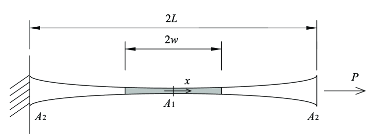
Figure 3: Quadratically tapering bar.

Considering that the origin is located as the centre of the bar, the cross section $A$ is given by

$$A(x)=A_{1}+\gamma^{2}A_{1}\frac{x^{2}}{L^{2}},$$ (51)

where $\gamma$ controls the ratio between $A_{1}$ and $A_{2}$ ($\gamma^{2}=\left({A_{2}-A_{1}}\right)/A_{1}$). This problem can be equivalently formulated as a rod with unit cross-section and loading $f$ which varies along the rod, which allows the convergence analysis from the previous section to be carried over for this case. The exact solution for $\varepsilon$ along the bar is:

$$\varepsilon=\frac{PL^{2}}{EA_{1}\left({L^{2}+\gamma^{2}x^{2}}\right)},$$ (52)

and the exact solution of $\varepsilon_{,xx}$ is:

$$\varepsilon_{,xx}=\frac{2PL^{2}\gamma^{2}\left({3\gamma^{2}x^{2}-L^{2}}\right)}{EA_{1}\left({L^{2}+\gamma^{2}x^{2}}\right)^{3}}.$$ (53)

The term $\overline{\varepsilon}^{h}$ involves both $\varepsilon$ and $\varepsilon_{,xx}$. The $\varepsilon$ component involves the standard $L^{2}$ projection of $\varepsilon^{h}$ (coming from the solution of the equilibrium equation) onto the basis for $\overline{\varepsilon}^{h}$. This projection does not involve any of the element interface terms that have arisen in the discontinuous Galerkin formulation. Of special interest is the approximation of the $\varepsilon_{,xx}$ term. To examine numerically the convergence of this term, the weak form corresponding to:

$$\overline{\varepsilon}-\varepsilon_{,xx}=0$$ (54)

is solved, as it is the $\varepsilon_{,xx}$ term that dominates the convergence rate. However, in practice, the convergence rate of $\varepsilon$ may appear to dominate due to a large difference in the constants in the error inequality. Taking equation (22) and removing terms related to the projection of $\varepsilon^{h}$, we solve the following problem: find $u^{h}\in\mathcal{S}^{h}$ and $\overline{\varepsilon}^{h}\in\mathcal{W}^{h}$ such that

$$\int_{\Omega}w^{h}_{,x}Eu^{h}_{,x}\ d\Omega-w^{h}P|_{x=L}=0\quad\forall\ w^{h}\in\mathcal{V}^{h},$$ (55)

$$\int_{\Omega}q^{h}\overline{\varepsilon}^{h}\ d\Omega+\int_{\widetilde{\Omega}}q^{h}_{,x}\varepsilon^{h}_{,x}\ d\Omega-\int_{\Gamma}q^{h}\varepsilon_{,x}^{h}n\ d\Gamma-\int_{\widetilde{\Gamma}}\left\llbracket{q^{h}}\right\rrbracket\left<{\varepsilon^{h}_{,x}}\right>\ d\Gamma\\ -\int_{\widetilde{\Gamma}}\left<{q^{h}_{,x}}\right>\left\llbracket{\varepsilon^{h}}\right\rrbracket\ d\Gamma+\int_{\widetilde{\Gamma}}\frac{\alpha}{h}\left\llbracket{q^{h}}\right\rrbracket\left\llbracket{\varepsilon^{h}}\right\rrbracket\ d\Gamma=0\quad\forall\ q^{h}\in\mathcal{W}^{h}.$$ (56)

For the parameters $A_{1}=1$ mm², $A_{2}=0.1$ mm², $L=50$ mm, $E=1$ MPa and $P=1$ N, the convergence behaviour is examined for a range of elements. To gain insight, the form of the exact solution is shown in Figure 4.

\psfrag{x}{$x$}\psfrag{y}{$\varepsilon_{,xx}$}\includegraphics{eps_xx_elastic.eps}

Figure 4: Exact solution for $\varepsilon_{,xx}$.

The $L^{2}$-norm of the computed error for a range elements is shown in Figure 5 for the case $\alpha=1$.

\psfrag{x}{$n_{\rm el}$}\psfrag{y}{$\|\varepsilon_{,xx}-\overline{\varepsilon}^{h}\|$}\psfrag{P10d}{{\tiny$P^{1}/P^{0}(C^{-1})$}}\psfrag{P21c}{{\tiny$P^{2}/P^{1}(C^{0})$}}\psfrag{P21d}{{\tiny$P^{2}/P^{1}(C^{-1})$}}\psfrag{P32c}{{\tiny$P^{3}/P^{2}(C^{0})$}}\psfrag{P32d}{{\tiny$P^{3}/P^{2}(C^{-1})$}}\includegraphics{eps_xx_conv_elastic_100.eps}

Figure 5: Convergence for the problem $\overline{\varepsilon}=\varepsilon_{,xx}$ with $\alpha=1$ on the domain $-50<x<50$.

If the error is computed by integrating over the entire bar ($-50<x<50$), as in Figure 5, the results are polluted by errors at the boundaries of the bar. In Figure 5, the convergence behaviour represents primarily how rapidly the computed solution approaches the exact solution at the boundaries. However, when simulating a tapered damaging bar, the error at the boundaries of the bar is of little consequence as damage develops at the centre, and $\overline{\varepsilon}$ at the boundaries plays no role (presuming that the deviation from the exact solution is not sufficient to induce spurious damage development). Excluding the error at the end of the bar by integrating over $-40<x<40$, the convergence behaviour is more predictable, as can be seen in Figure 6.

\psfrag{x}{$n_{\rm el}$}\psfrag{y}{$\|\varepsilon_{,xx}-\overline{\varepsilon}^{h}\|$}\psfrag{P10d}{{\tiny$P^{1}/P^{0}(C^{-1})$}}\psfrag{P21c}{{\tiny$P^{2}/P^{1}(C^{0})$}}\psfrag{P21d}{{\tiny$P^{2}/P^{1}(C^{-1})$}}\psfrag{P32c}{{\tiny$P^{3}/P^{2}(C^{0})$}}\psfrag{P32d}{{\tiny$P^{3}/P^{2}(C^{-1})$}}\includegraphics{eps_xx_conv_elastic_90.eps}

Figure 6: Convergence for the problem $\overline{\varepsilon}=\varepsilon_{,xx}$ with $\alpha=1$ on the domain $-40<x<40$.

From Figure 6, it can be concluded that the convergence rate for all elements is consistent with the predicted rates (as summarised in Table 1).

The effect of $\alpha$ on convergence for the $P^{2}/P^{1}\left({C^{-1}}\right)$ element is shown in Figure 7.

\psfrag{x}{$n_{\rm el}$}\psfrag{y}{$\|\varepsilon_{,xx}-\overline{\varepsilon}^{h}\|$}\psfrag{aaaa1}{{\tiny$\alpha=1$}}\psfrag{aaaa2}{{\tiny$\alpha=2$}}\psfrag{aaaa3}{{\tiny$\alpha=3$}}\psfrag{aaaa4}{{\tiny$\alpha=4$}}\psfrag{aaaa5}{{\tiny$\alpha=5$}}\includegraphics{eps_xx_conv_elastic_90_d_alpha.eps}

Figure 7: Convergence of the $P^{2}/P^{1}\left({C^{-1}}\right)$ element for different values of $\alpha$ on the domain $-40<x<40$ for the problem $\overline{\varepsilon}=\varepsilon_{,xx}$.

As expected, the convergence rate is unaffected by $\alpha$. For the $P^{3}/P^{2}\left({C^{-1}}\right)$ element, the convergence behaviour for different $\alpha$ is shown in Figure 8.

\psfrag{x}{$n_{\rm el}$}\psfrag{y}{$\|\varepsilon_{,xx}-\overline{\varepsilon}^{h}\|$}\psfrag{aaaa1}{{\tiny$\alpha=1$}}\psfrag{aaaa2}{{\tiny$\alpha=2$}}\psfrag{aaaa4}{{\tiny$\alpha=4$}}\psfrag{aaa55}{{\tiny$\alpha=5.5$}}\psfrag{aaa58}{{\tiny$\alpha=5.8$}}\psfrag{aaaa6}{{\tiny$\alpha=6$}}\psfrag{aaa62}{{\tiny$\alpha=6.2$}}\psfrag{aaa65}{{\tiny$\alpha=6.5$}}\includegraphics{eps_xx_conv_elastic_90_d_alpha_32.eps}

Figure 8: Convergence of the $P^{3}/P^{2}\left({C^{-1}}\right)$ element for different values of $\alpha$ on the domain $-40<x<40$ for the problem $\overline{\varepsilon}=\varepsilon_{,xx}$.

From Figure 8, it is clear the convergence rate increases by one order for $\alpha=6$. This is close to the predicted value of $\alpha=5.5$.

4.2 Convergence for the inelastic case in one dimension

The formulation is now examined for the inelastic case. Again, the quadratically tapering bar is considered, which leads to damage development at the centre of the bar. For a particular relationship between $D$ and $\kappa$, it is possible to solve the problem analytically, which provides the basis for numerical convergence tests.

4.2.1 Analytical solution

Consider again the bar shown in Figure 3, where the shaded region indicates the damaged zone and $x=\pm w$ is the location of the damage–elastic boundary. For convenience, the force $P$ is expressed as

$$P=\left({1-\beta^{2}}\right)EA_{1}\kappa_{0},$$ (57)

where $\beta$ governs the magnitude of the applied load and $\kappa_{0}$ is the value of $\kappa$ at which damage is first induced. In the undamaged part of the bar, the strain response is given by

$$\varepsilon=\dfrac{P}{EA},$$ (58)

and within the damaged zone by,

$$\varepsilon=\dfrac{P}{\left({1-D}\right)EA}.$$ (59)

With the intention of finding an analytical solution, a simple damage law is assumed,

$$D=\begin{cases}0&{\rm if}\ \kappa\leq\kappa_{0}\\ 1-\dfrac{\kappa_{0}}{\kappa}&{\rm if}\ \kappa>\kappa_{0}.\end{cases}$$ (60)

The relationship in equation (60) is the analogy of perfect plasticity for the case $c=0$, in the sense that it yields a plateau in the load–displacement response once the elastic limit has been exceeded. Assuming that no unloading takes place in the damaged zone, $\kappa=\overline{\varepsilon}$, that is

$$\kappa=\varepsilon+c^{2}\varepsilon_{,xx}\quad-w<x<w.$$ (61)

Inserting equations (61) and (60) into equation (59), the following ordinary differential equation is obtained:

$$\left({1-\dfrac{P}{\kappa_{0}EA}}\right)\varepsilon-c^{2}\dfrac{P}{\kappa_{0}EA}\varepsilon_{,xx}=0\quad-w<x<w,$$ (62)

which governs the response in the damaged zone. The general solution to the above equation for $x>0$ is given by:

$$\varepsilon=C_{1}\frac{M\left({\frac{\beta^{2}L}{4c\gamma\sqrt{1+\beta^{2}}},\dfrac{1}{4},\frac{\gamma x^{2}}{Lc\sqrt{1+\beta^{2}}}}\right)}{\sqrt{x}}+C_{2}\frac{W\left({\frac{\beta^{2}L}{4c\gamma\sqrt{1+\beta^{2}}},\dfrac{1}{4},\frac{\gamma x^{2}}{Lc\sqrt{1+\beta^{2}}}}\right)}{\sqrt{x}},$$ (63)

where $M$ and $W$ are Whittaker’s functions (Abramowitz and Stegun, 1965), and $C_{1}$ and $C_{2}$ are integration constants. The integration constants can be obtained by considering boundary conditions at $x=\pm w$. The first considered condition is symmetry about $x=0$. Expanding equation (63) in a Taylor series about $x=0$, and requiring that odd terms vanish, the following relation is obtained:

$$C_{1}=C_{2}\frac{2\pi}{\Gamma\left({\frac{1}{4}-\frac{-\beta^{2}L^{2}+c\gamma\sqrt{1+\beta^{2}}}{4c\sqrt{1+\gamma\beta^{2}}}}\right)},$$ (64)

where $\Gamma$ is the Gamma function. The second considered condition is:

$$\left\llbracket{\varepsilon_{,x}}\right\rrbracket=0\quad{\rm at}\ x=w,$$ (65)

which implies

$$\varepsilon_{,x}=\left({\frac{P}{EA}}\right)_{,x}\quad{\rm at}\ x=w.$$ (66)

Finally, the location of the elastic–damage boundary can be determined by requiring that

$$\kappa=\kappa_{0}\quad{\rm at}\ x=w.$$ (67)

For the sake of brevity, the expressions for $C_{1}$, $C_{2}$ and $w$ have been omitted.

4.2.2 Damage convergence results

The convergence behaviour of various elements for the outlined test problem is now examined. For the tests, the following parameters are adopted: $\gamma=3$, $\beta=5/29$, $L=100$ mm, $E=200\times 10^{3}$ MPa, $c=1$ mm and $A_{1}=1$ mm² and $\kappa_{0}=1\times 10^{-3}$. In calculating the error, the Gamma function has been computed numerically.

The results of the error analysis, for various elements, are shown in Figure 9.

\psfrag{x}{$n_{\rm el}$}\psfrag{y}{$\|\varepsilon-\varepsilon^{h}\|$}\psfrag{P10d}{{\tiny$P^{1}/P^{0}(C^{-1})$}}\psfrag{P21c}{{\tiny$P^{2}/P^{1}(C^{0})$}}\psfrag{P21d}{{\tiny$P^{2}/P^{1}(C^{-1})$}}\psfrag{P32c}{{\tiny$P^{3}/P^{2}(C^{0})$}}\psfrag{P32d}{{\tiny$P^{3}/P^{2}(C^{-1})$}}\includegraphics{eps_conv_dam.eps}

Figure 9: Error in $\varepsilon^{h}$ for the damaging bar.

For the $P^{1}/P^{0}\left({C^{-1}}\right)$, $P^{2}/P^{1}\left({C^{-1}}\right)$ and $P^{3}/P^{2}\left({C^{-1}}\right)$ elements, $\alpha=1$, $\alpha=4$ and $\alpha=6$, respectively. These choices draw upon the observed convergence results for the elastic case. For all the elements, the solution converges. Once a level of refinement has been reached, the convergence rate is linear. Moreover, for a given interpolation order, continuous and discontinuous interpolations yield similar results.

4.2.3 Non-trivial damage response

The quadratically tapering bar is now examined for a non-trivial softening relationship. For the tapered bar the relevant parameters are: $\gamma=3$, $A_{1}=1$ mm², Young’s modulus $E=20\times 10^{3}$ MPa, $\kappa_{0}=1\times 10^{-4}$, $\kappa_{c}=0.0125$, and $c=1$ mm. The functional form of the damage variable is specified to be

$$D=\begin{cases}0&{\rm if}\ \kappa\leq\kappa_{0}\\ 1-\dfrac{\kappa_{0}(\kappa_{c}-\kappa)}{\kappa(\kappa_{c}-\kappa_{0})}&{\rm if}\ \kappa_{0}<\kappa<\kappa_{c}\\ 1&{\rm if}\ \kappa\geq\kappa_{c},\end{cases}$$ (68)

which leads to a linear softening relationship for $c=0$. The numerical performance of the formulation has previously been demonstrated in Wells et al. (2004) for continuous, piecewise linear $u^{h}$ and constant $\overline{\varepsilon}^{h}$, discontinuous across element boundaries (the $P^{1}/P^{0}(C^{-1})$ element). The formulation was shown numerically to converge to a benchmark solution. Here, the formulation is extended for a range of different element types.

The motivation behind the considered strain gradient-dependent model is regularisation in the presence of strain softening. Without strain gradient effects ($c=0$), computed results are pathologically mesh-dependent; the result of which is manifest in the load–displacement responses. Therefore, each of the elements which to this point have been examined are tested, and the load-displacement responses reported for meshes with 20, 40, 80, 160 and 320 elements. For the $P^{3}/P^{2}(C^{-1})$ element, the numerical tests are performed with meshes of 20, 40, 80 and 160 elements. To provide a reference solution, the response computed using 160 $P^{3}/P^{2}\left({C^{0}}\right)$ elements is included in all figures.

The load-displacement responses for the two elements using a continuous interpolation of $\overline{\varepsilon}^{h}$ are shown in Figure 10.

\psfrag{x}{$u$}\psfrag{y}{$P$}\includegraphics{PU_P1P0.eps}

(a)

\psfrag{x}{$u$}\psfrag{y}{$P$}\includegraphics{PU_P2P1c.eps}

(b)

Figure 10: Load–displacement response for (a) $P^{2}/P^{1}\left({C^{0}}\right)$ and (b) $P^{3}/P^{2}\left({C^{0}}\right)$ elements.

As the mesh is refined, the computed response for both element types converges towards to the reference solution. The load-displacement responses for three elements using a discontinuous interpolation of $\overline{\varepsilon}^{h}$ are shown in Figure 11. Again, for the $P^{1}/P^{0}\left({C^{-1}}\right)$ element, $\alpha=1$, for the $P^{2}/P^{1}\left({C^{-1}}\right)$ element, $\alpha=4$, and for the $P^{3}/P^{2}\left({C^{-1}}\right)$ element, $\alpha=6$.

\psfrag{x}{$u$}\psfrag{y}{$P$}\includegraphics{PU_P1P0.eps}

(a)

\psfrag{x}{$u$}\psfrag{y}{$P$}\includegraphics{PU_P2P1d.eps}

(b)

\psfrag{x}{$u$}\psfrag{y}{$P$}\includegraphics{PU_P3P2d.eps}

(c)

Figure 11: Load–displacement response for (a) $P^{1}/P^{0}\left({C^{-1}}\right)$, (b) $P^{2}/P^{1}\left({C^{-1}}\right)$ and (c) $P^{3}/P^{2}\left({C^{-1}}\right)$ elements.

It is clear, for all elements, that the load–displacement response converges to the reference solution with mesh refinement. To further examine the computed results, the damage profiles for the two continuous elements and the three discontinuous elements are compared in Figures 12 and 13, respectively. For all cases, the 160 element mesh is considered.

\psfrag{x}{$x$}\psfrag{y}{$D$}\psfrag{aaaaaP2P1c}{\tiny$P^{2}/P^{1}(C^{0})$}\psfrag{aaaaaP3P2c}{\tiny$P^{3}/P^{2}(C^{0})$}\includegraphics{damage_profile_cont.eps}

Figure 12: Damage profiles for the $\overline{\varepsilon}^{h}$-continuous elements, computed using 160 elements.

\psfrag{x}{$x$}\psfrag{y}{$D$}\psfrag{aaaaaP1P0d}{\tiny$P^{1}/P^{0}(C^{-1})$}\psfrag{aaaaaP2P1d}{\tiny$P^{2}/P^{3}(C^{-1})$}\psfrag{aaaaaP3P2d}{\tiny$P^{3}/P^{2}(C^{-1})$}\includegraphics{damage_profile_disc.eps}

Figure 13: Damage profiles for the $\overline{\varepsilon}^{h}$-discontinuous elements, computed using 160 elements.

Clearly, the damage profiles are nearly identical for all element types.

4.3 Three-point bending test

To conclude the numerical validations, a three-point bending test is performed using a $P^{2}/P^{1}\left({C^{0}}\right)$ element. The element is triangular, with degrees of freedom for $\bm{u}^{h}$ located at the vertexes and at the mid-sides, and degrees of freedom for $\overline{\varepsilon}^{h}$ located only at the vertexes of the element. The choice of a quadratic interpolation of $\bm{u}^{h}$ means that the penalty term for imposing the non-standard boundary condition in equation (21) vanishes, and the non-standard boundary condition is satisfied by construction (see equation (21)). The equivalent strain is taken as the trace of the strain tensor,

$$\varepsilon^{\rm eq}={\rm trace}\left({\bm{\varepsilon}}\right).$$ (69)

This choice does not reflect a strong physical motivation, rather it is chosen for illustrative purposes as it allows for relatively simple linearisation of the method (which can become extremely complex when $c\neq 0$).

The three-point bending test is performed for two different meshes with $c\neq 0$ and $c=0$. The adopted geometry for the three-point bending test is shown in Figure 14, and the adopted material parameters are: Young’s modulus $E=20\times 10^{4}$ MPa, Poisson’s ratio $\nu=0$, $\kappa_{0}=1\times 10^{-4}$, and $\kappa_{c}=1.25\times 10^{-2}$. For gradient-dependent simulations, $c=8\times 10^{-2}$ mm.

Figure 14: Three-point bending specimen.

Computations are stopped when damage reaches unity at any point in the mesh, and damage development at the supports is prevented. The computed damage contours for the four cases are shown in Figure 15.

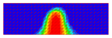
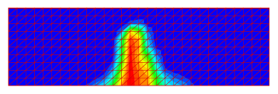
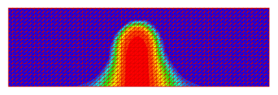
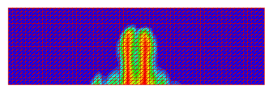
(a)	(b)

Figure 15: Damage contours for two meshes (a) with gradient effects ($c\neq 0$) and (b) without gradient effects ($c=0$).

From the damage contours, it is clear that the computed results are similar for the two meshes with $c\neq 0$. In the absence of regularising effects ($c=0$), the result is clearly affected by the discretisation. The load–displacement responses for the various cases are shown in Figure 16. Recall that a computation is halted when damage reaches unity at a material point. For the gradient-dependent case, the responses for the two meshes are similar. For the case $c=0$, the responses are also similar, which is somewhat in contrast to what is normally expected for a strain softening problem. The responses are similar in this case due to the spurious development of two cracks for the finer mesh (in contrast to the single main crack for the coarse mesh). This is evident from the damage contours in Figure 15.

\psfrag{x}{$u$}\psfrag{y}{$P$}\psfrag{coarseaaaaaa}{\tiny coarse $c=0$}\psfrag{caorsecaaaaa}{\tiny coarse $c\neq 0$}\psfrag{fineaaaaaaaa}{\tiny fine $c=0$}\psfrag{finecaaaaaaa}{\tiny fine $c\neq 0$}\includegraphics{Pu_2d.eps}

Figure 16: Load–displacement responses for two different meshes.

5 Conclusions

A discontinuous Galerkin formulation for a strain gradient-dependent damage model has been investigated for a range of different finite elements. The model allows the numerical solution of a continuum problem which would classically require $C^{1}$ interpolations with a simple $C^{0}$ or even discontinuous basis. Examples demonstrate robust performance for a range of polynomial orders and degrees of continuity of the interpolation functions, and are supported by rigorous error analysis. Specifically, lower-order interpolations perform well and are relatively simple to construct. The convergence properties of the proposed method have been examined for the elastic case, for which the observed rates are consistent with the theoretically predicted rates. The formulation has been observed numerically to converge also for damage problems. Finally, the formulation was applied successfully to a two-dimensional problem. While the approach is promising, several issues remain. Difficulties which must be resolved for other gradient models include the effective imposition of boundary conditions on the fixed boundary of a body, and at moving boundaries internal to a body. The development of thermodynamically consistent models would assist in this sense, as the higher-order kinematic gradients have a natural partner in the energetic sense.

References

- Abramowitz and Stegun (1965) Abramowitz, M., Stegun, I. A. (Eds.), 1965. Handbook of Mathematical Functions. Dover Publications, Inc., New York.
- Aifantis (1984) Aifantis, E. C., 1984. On the microstructural origin of certain inelastic models. Journal of Engineering Materials Technology 106, 326–334.
- Arnold et al. (2002) Arnold, D. N., Brezzi, F., Cockburn, B., Marini, D., 2002. Unified analysis of discontinuous Galerkin methods for elliptic problems. SIAM Journal on Numerical Analysis 39 (5), 1749–1779.
- Askes et al. (2000) Askes, H., Pamin, J., de Borst, R., 2000. Dispersion analysis and element-free Galerkin solutions of second- and fourth-order gradient-enhanced damage models. International Journal for Numerical Methods in Engineering 69 (6), 811–832.
- Bažant (1986) Bažant, Z. P., 1986. Mechanics of distributed cracking. Applied Mechanics Reviews 39, 675–705.
- Bažant and Oh (1983) Bažant, Z. P., Oh, B., 1983. Crack band theory for fracture of concrete. RILEM Materials and Structures 16 (93), 155–177.
- Bažant and Pijaudier-Cabot (1988) Bažant, Z. P., Pijaudier-Cabot, G., 1988. Nonlocal continuum damage, localization instability and convergence. Journal of Applied Mechanics 55, 287–293.
- Borino et al. (2003) Borino, G., Failla, B., Parrinello, F., 2003. A symmetric nonlocal damage theory. International Journal of Solids and Structures 40, 3621–3645.
- Coleman and Hodgdon (1985) Coleman, B. D., Hodgdon, M. L., 1985. On shear bands in ductile materials. Archives for Rational Mechanics and Analysis 90, 219–247.
- de Borst and Sluys (1991) de Borst, R., Sluys, L. J., 1991. Localisation in a Cosserat continuum under static and dynamic loading conditions. Computer Methods in Applied Mechanics and Engineering 90, 805–827.
- de Vree et al. (1995) de Vree, J. H. P., Brekelmans, W. A. M., van Gils, M. A. J., 1995. Comparison of non-local approaches in continuum damage mechanics. Computers and Structures 55 (4), 581–588.
- Engel et al. (2002) Engel, G., Garikipati, K., Hughes, T. J. R., Larson, M. G., Mazzei, L., Taylor, R. L., 2002. Continuous/discontinuous finite element approximations of fourth-order elliptic problems in structural and continuum mechanics with applications to thin beams and plates, and strain gradient elasticity. Computer Methods in Applied Mechanics and Engineering 191 (34), 3669–3750.
- Kachanov (1958) Kachanov, L. M., 1958. On creep rupture time. IZV Akad Nauk SSSR Otd. Tech. Nauk 8, 26–31.
- Lasry and Belytchko (1998) Lasry, D., Belytchko, T., 1998. Localization limiters in transient problem. International Journal of Solids and Structures 24 (6), 581–597.
- Oden and Carey (1984) Oden, J. T., Carey, G. F., 1984. Finite Elements: Mathematical Aspects. Volume IV. Prentice-Hall, Englewood Cliffs, N.J.
- Peerlings et al. (1996) Peerlings, R. H. J., de Borst, R., Brekelmans, A. M., de Vree, J. H. P., 1996. Gradient enhanced damage for quasi-brittle materials. International Journal for Numerical Methods in Engineering 39, 3391–3403.
- Rashid (1968) Rashid, Y. R., 1968. Ultimate strength analysis of prestressed concrete pressure vessels. Nuclear Engineering and Design 7, 334–344.
- Rice (1976) Rice, J. R., 1976. The localization of plastic deformation. In: Koiter, W. T. (Ed.), Theoretical and Applied Mechanics. North Holland Publishing Co., pp. 207–220.
- Shu et al. (1999) Shu, J. Y., King, W. E., Fleck, N. A., 1999. Finite elements for materials with strain gradient effects. International Journal for Numerical Methods in Engineering 44, 373–391.
- Strang and Fix (1973) Strang, G., Fix, G. J., 1973. An Analysis of the Finite Element Method. Prentice-Hall, New Jersey.
- Triantafyllidis and Aifantis (1986) Triantafyllidis, N., Aifantis, E. C., 1986. A gradient approach to localization of deformation: I hyperelastic materials. Journal of Elasticity 16, 225–237.
- Wells et al. (2004) Wells, G. N., Garikipati, K., Molari, L., 2004. A discontinuous Galerkin formulation for a strain gradient-dependent continuum model. Computer Methods in Applied Mechanics and Engineering 193 (33-35), 3633–3645.
- Willam (1984) Willam, K., 1984. Experimental and computational aspects of concrete fracture. In: Owen, R., Hinton, E., Bićanić (Eds.), Proc. Int. Conf. Comp. Aided Anal. and Design of Concrete Structures. Pineridge Press, Swansea, U.K., pp. 33–70.
- Zervos et al. (2001) Zervos, A., Papanastasiou, P., Vardoulakis, I., 2001. A finite element displacement formulation for gradient elastoplasticity. International Journal for Numerical Methods in Engineering 50, 1369–1388.