Impurity Transport in Plasma Edge Turbulence

The turbulent transport of minority species/impurities is investigated in 2D drift-wave turbulence as well as in 3D toroidal drift-Alfvén edge turbulence. The full effects of perpendicular and – in 3D – parallel advection are kept for the impurity species. Anomalous pinch effects are recovered and explained in terms of Turbulent EquiPartition (TEP)

1 Anomalous Pinch in 2D Drift-Wave Turbulence

The Hasegawa-Wakatani model [1] for 2D resistive drift-wave turbulence reads

$$\lx@equationgroup@subnumbering@begin d_{t}{(n-x)}=\mathcal{C}(\varphi-n)+\mu_{n}\nabla_{\perp}^{2}n,\hskip 8.61108ptd_{t}{\omega}=\mathcal{C}(\varphi-n)+\mu_{\omega}\nabla_{\perp}^{2}\omega,\lx@equationgroup@subnumbering@end$$ (2)

with $\omega\equiv\nabla_{\perp}^{2}\varphi$ and $d_{t}\equiv\partial/\partial t+{\bf\hat{z}}\bm{\times}\bm{\nabla}_{\perp}\varphi\bm{\cdot}\bm{\nabla}_{\perp}$. Here, $n$ and $\varphi$ denote fluctuations in density and electrostatic potential. $\omega$ is the vorticity, $\nabla\times{\bf\hat{z}}\bm{\times}\bm{\nabla}_{\perp}\varphi$. The parameters in the HW system are the parallel coupling $\mathcal{C}$, and diffusivities, $\mu_{n}$,$\mu_{\omega}$.
2D impurity transport in magnetized plasma is modeled by the transport of a passive scalar field:

$$d_{t}{\theta}-\zeta\bm{\nabla}_{\perp}\bm{\cdot}\bigg{(}\theta d_{t}{\bm{\nabla}_{\perp}\varphi}\bigg{)}=\mu_{\theta}\nabla_{\perp}^{2}\theta,$$ (3)

where $\theta$ is the density of impurities, $\mu_{\theta}$ the collisional diffusivity, and $\zeta=\frac{m_{\theta}}{q_{\theta}}\frac{e}{m_{i}}\frac{\rho_{s}}{L_{n}}$ the influence of inertia, which enters via the polarization drift. The latter makes the flow compressible, consequently for ideal (massless) impurities, $\zeta=0$ and advection is due to the incompressible electric drift only. In all cases the impurity density is assumed to be so low compared to the bulk plasma density that there is no back-reaction on the bulk plasma dynamics.

1.1 Vorticity - Impurity correlation

The equation for the impurities can be rewritten in the form:

$$d_{t}{(\ln\theta-\zeta\omega)}=\zeta\bm{\nabla}_{\perp}\ln\theta\bm{\cdot}d_{t}{\bm{\nabla}_{\perp}\varphi}+\frac{\mu_{\theta}}{\theta}\,\nabla_{\perp}^{2}\theta\;.$$

If the diffusivity $\mu_{\theta}$ is of order $\zeta\ll 1$ and fluctuations $\theta_{1}$ of the impurity density measured relative to a constant impurity background $\theta_{0}$ do not exceed a corresponding level, the quantity $\ln\theta-\zeta\omega$ is approximately a Lagrangian invariant. Turbulent mixing will homogenize Lagrangian invariants in TEP states [2, 3], leading to

$$\ln\theta-\zeta\omega\approx\mathrm{const},$$

which constitutes a prediction about the effect of compressibility on the initially homogeneous impurity density field. The conservation of impurity density yields

$$\frac{\theta}{\theta_{0}}\approx 1+\zeta\omega,$$

which conforms with the assumed ordering. We thus predict a linear relation between impurity density $\theta$ and vorticity $\omega$, the proportionality constant being the mass–charge ratio $\zeta$. This is related, but not the same as, to the aggregation of dense particles in vortices in fluids due to the Coriolis force [4].

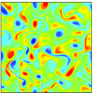
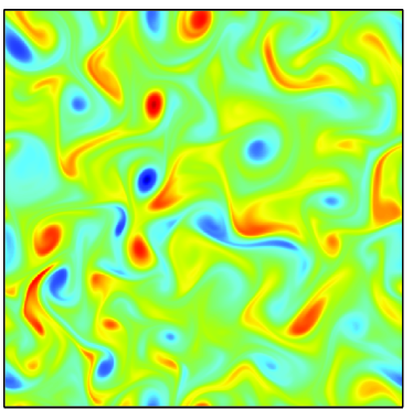
Figure 1: (a) Vorticity and (b) density of inertial impurities in the saturated state with $\mathcal{C}=1$ and $\zeta=0.01$, L = 40. Other parameters: $\mu_{n}=\mu_{\omega}=\mu_{\theta}=0.02$.

The prediction is verified by numerical simulations of inertial impurities in saturated HW-turbulence for $\mathcal{C}=1$. The simulations are performed on a $[-20,20]^{2}$ domain, using $512^{2}$ gridpoints, and impurity diffusivity $0.02$. The impurity density field is initially set to unity. The impurity density field for $\zeta=0.01$ is presented together with vorticity in Figure 1. Figure 3 shows a scatter plot of the point values of impurity density and vorticity at time $150$ for three different values of $\zeta$. The proportionality factor $\theta=1+K\omega$ is determined to be slightly below one: $K\simeq 0.82\,\zeta$.

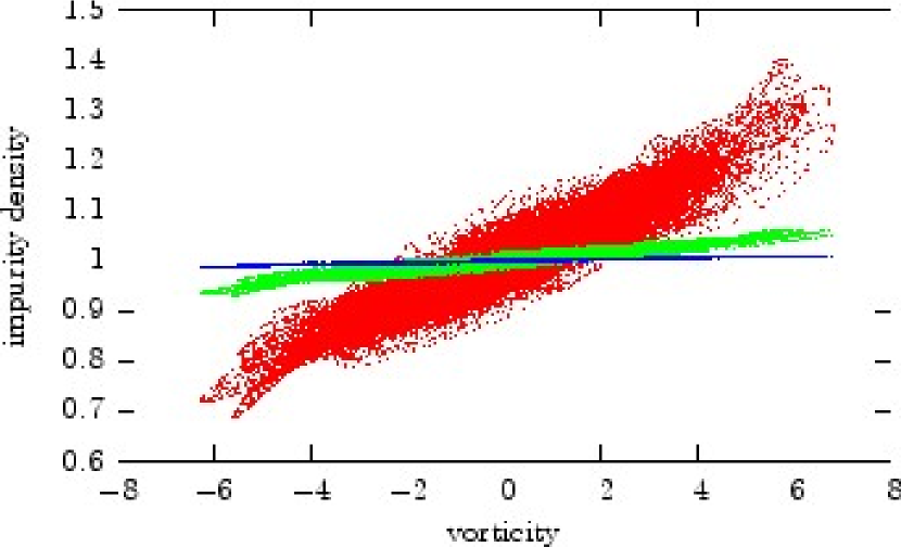
Figure 2: Scatter plot of impurity density and the vorticity field at $t=100$ for different values of the mass–charge ratio $\zeta$ in the saturated state in HW with $\mathcal{C}=1$: $\zeta=0.05$ (red), $\zeta=0.01$ (green), and $\zeta=0.002$ (blue).

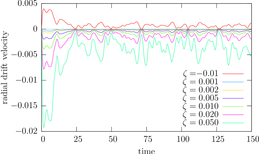
Figure 3: Evolution of the radial drift velocity of inertial impurities in the saturated state in HW with $\mathcal{C}=1$. The impurities are uniformly distributed at $t=0$.

1.2 Anomalous pinch

The role of inertia for a radially inward pinch is investigated by considering the collective drift of impurities. Ideal impurities do on average not experience a drift, but this is not the case for inertial impurities, since compressibility effects arrange for a correlation between $\theta_{1}$ and $\omega$. Note that only the deviations from the above discussed linear relationship $\theta=1+K\omega$ result in a net flow, as $\int K\omega v_{r}\,dx=0$ for periodic boundary conditions.

The evolution of the radial drift velocity, measured as the net radial impurity transport, is presented in Figure 3. The radial drift velocity has a definite sign that depends on the sign of $\zeta$. There is a continuous flow of impurities in a definite direction (inward for positively charged impurities). This resembles the anomalous pinch observed in magnetic confinement experiments [5]. Average radial drift velocities computed using the values of the drift from $t=25$ to $t=150$ are presented in Table 1. The scaling of the average radial drift with $\zeta$ is seen to be remarkably linear.

Table 1: Radial drift velocity of impurities for different values of the mass–charge ratio $\zeta$ in the saturated state in HW with $\mathcal{C}=1$. Calculated as the average value between $t=25$ and $t=150$. Parameters: $\mu_{n}=\mu_{\omega}=\mu_{\theta}=0.02$.

$\zeta$	radial drift
$-0.010$	$\phantom{-}8.67\times 10^{-4}$
$0.001$	$-8.66\times 10^{-5}$
$0.002$	$-1.73\times 10^{-4}$
$0.005$	$-4.35\times 10^{-4}$
$0.010$	$-8.69\times 10^{-4}$
$0.020$	$-1.75\times 10^{-3}$
$0.050$	$-4.55\times 10^{-3}$

2 Drift-Alfvén Turbulence

We now consider drift-Alfvén turbulence in flux tube geometry  [6, 7, 8]. The following equations for the fluctuations in density $n$, potential $\phi$ with associated vorticity $\omega=\nabla_{\perp}^{2}\phi$, current $J$ and parallel ion velocity $u$ arise in the usual drift-scaling:

$$\frac{\partial\omega}{\partial t}+\{\phi,\omega\}=\mathcal{K}\left(n\right)+\nabla_{\shortparallel}J+\mu_{\omega}\nabla_{\perp}^{2}\omega,$$ (4a)

$$\frac{\partial n}{\partial t}+\{\phi,n_{EQ}+n\}=\mathcal{K}\left(n-\phi\right)+\nabla_{\shortparallel}\left(J-u\right)+\mu_{n}\nabla_{\perp}^{2}n,$$ (4b)

$$\frac{\partial}{\partial t}\left(\widehat{\beta}A_{\shortparallel}+\widehat{\mu}J\right)+\widehat{\mu}\left\{\phi,J\right\}=\nabla_{\shortparallel}\left(n_{EQ}+n-\phi\right)-CJ,$$ (4c)

$$\widehat{\epsilon}\left(\frac{\partial u}{\partial t}+\left\{\phi,u\right\}\right)=-\nabla_{\shortparallel}\left(n_{EQ}+n\right).$$ (4d)

The evolution of the impurity density is given by

$$d_{t}\theta=(\zeta/\widehat{\epsilon})\nabla_{\perp}\cdot\left(\theta d_{t}\nabla_{\perp}\phi\right)-\theta\mathcal{K}\left(\phi\right)-\nabla_{\|}\left(\theta u\right)-\mu_{\theta}\nabla_{\perp}^{2}\theta$$ (5)

Standard parameters for simulation runs were $\widehat{\mu}=5$, $q=3$, magnetic shear $\widehat{s}=1$, and $\omega_{B}=0.05$, with $\mu_{\omega}=\mu_{n}=0.025$, corresponding to typical edge parameters of large fusion devices. Simulations were performed on a grid with $128\times 512\times 32$ points and dimensions $64\times 256\times 2\pi$ in ${x,y,s}$ corresponding to a typical approximate dimensional size of 2.5 cm $\times$ 10 cm$\times$ 30 m [6]. Here we present results from a low $\hat{\beta}=0.1$ run with $C=11.5$. In Figure 4 the dynamical evolution of the impurity density is exemplified in a plot showing the poloidal projection of the impurity density.
The flux $\Gamma$ of the impurity ion species can in lowest order be expressed by the standard parameters used in modeling and in evaluation of transport experiments: a diffusion coefficient $D$ and a velocity $V$, which is associated to a pinch effect,

$$\Gamma_{y}(s)=-D(s)\partial_{x}\left<\theta\right>_{y}+V(s)\left<\theta\right>_{y}\,.$$ (6)

From scatter plots of $\Gamma(r)/\left<n\right>_{y}$ versus $\partial_{x}\ln\left<n\right>_{y}$, values for $D(s)$ and $V(s)$ are obtained. The poloidal (coordinate $s$) dependence of $D$ and $V$ is rather strong and shown, with numerical uncertainties, in Fig. 5. The effective advective velocity $V(s)$ changes sign and is at the high field side directed outwards. This pinching velocity is due to curvature and can be consistently explained in the framework of Turbulent EquiPartition (TEP) [9, 3] as follows: In the absence of parallel advection, finite mass effects and diffusion, Eq. (5) has the following approximate Lagrangian invariant

$$L(s)=\ln\theta+\omega_{B}x\cos(s)-\omega_{B}y\sin(s)\;.$$ (7)

TEP assumes the spatial homogenization of $L$ by the turbulence. As parallel transport is weak, each drift plane $s=\text{const.}$ homogenizes independently. This leads to profiles $\left<L(s)\right>_{y}=\text{const.}(s)$.

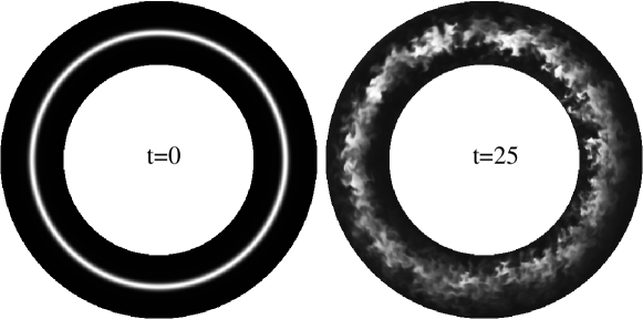
Figure 4: Impurity distribution projected onto a poloidal cross-section (radial dimension not to scale). Initial distribution (left) and after 25 time units (right).

At the outboard midplane ($s=0$) the impurites are effectively advected radially inward leading to an impurity profile ($\left<\ln\theta\right>_{y}\propto const.-\omega_{B}x$), while at the high field side they are effectively advected outward ($\left<\ln\theta\right>_{y}\propto const.+\omega_{B}x$). One should note that this effective inward or outward advection is not found as an average $E\times B$ velocity, but is mitigated by the effect of spatial homogenization of $L$ under the action of the turbulence. The strength of the “pinch” effect is consequently proportional to the mixing properties of the turbulence and scales with the measured effective turbulent diffusivity. We arrive at the following expression for the connection between pinch and diffusion:

$$V(s)=-\alpha\omega_{B}\cos(s)D(s)\;.$$ (8)

Considering a stationary case with zero flux and Eq. (7) we obtain $\alpha=1$. The ballooning in the turbulence level causes the inward flow on the outboard midplane to be stronger than the effective outflow on the high-field side. Therefore, averaged over a flux surface and assuming a poloidally constant impurity density, a net impurity inflow results. This net pinch is proportional to the diffusion coefficient $D$ in agreement with experimental observations [10].

Figure 5: Impurity diffusion $D$ (a) and pinch velocity $V$ (b) over poloidal position ($s$) with error-bars. The pinch velocity is compared to $\omega_{b}*\cos(s)*D(s)$ (dashed line).

Acknowledgement: Extensive discussions with O.E. Garcia are gratefully acknowledged.

References

- [1] A. Hasegawa and M. Wakatani, Phys. Rev. Lett. 50, 682 (1983).
- [2] V. V. Yan’kov, Physics-Uspekhi 40, 477 (1997).
- [3] V. Naulin, J. Nycander, and J. Juul Rasmussen, Phys. Rev. Lett. 81, 4148 (1998).
- [4] A. Bracco, P. H. Chavanis, A. Provenzale, and E. A. Spiegel, Phys. Fluids 11, 2280 (1999).
- [5] R. Dux, Fusion Science and Technology 44, 708 (2003).
- [6] B. D. Scott, Plasma Phys. Control. Fusion 39, 471 (1997).
- [7] B. D. Scott, Plasma Phys. Control. Fusion 39, 1635 (1997).
- [8] V. Naulin, Phys. Plasmas 10, 4016 (2003).
- [9] J. Nycander and V. V. Yan’kov, Phys. Plasmas 2, 2874 (1995).
- [10] M. E. Perry et al., Nucl. Fusion 31, 1859 (1991).