Kinetic fluctuation in the inhomogeneous plasma

Abstract

Using the Langevin approach and the multiscale technique, a kinetic theory of the time and space nonlocal fluctuations in the collisional plasma is constructed. In local equilibrium a generalized version of the Callen-Welton theorem is derived. It is shown that not only the dissipation but also the time and space derivatives of the dispersion determine the amplitude and the width of the spectrum lines of the electrostatic field fluctuations, as well as the form factor. There appear significant differences with respect to the non-uniform plasma. In the kinetic regime the form factor is more sensible to space gradient than the spectral function of the electrostatic field fluctuations. As a result of the inhomogeneity, these proprieties became asymmetric with respect to the inversion of the frequency sign. The differences in amplitude of peaks could become a new tool to diagnose slow time and space variations in the plasma.

PACS: 52.25.Dg; 52.25.Gj; 05.10.Gg; 05.40.-a

Keywords: Kinetic Theory; Plasma Fluctuations; Non-local Processes

Fluctuations find an application in diagnostic procedures. Indeed, plasma parameters such as temperature, mean velocity, density and their respective profiles can be determined by incoherent (Thomson) scattering diagnostics [1], i.e. by the proper interpretation of data obtained from the scattering of a given electromagnetic field interacting with the system. The key point of interpretating them is the knowledge of the intensity of the dielectric function fluctuations or equally of the electron form factor $(\delta n_{e}\delta n_{e})_{\omega,\mathbf{k}}$. Here $\omega$ and $\mathbf{k}$ are respectively the frequency and wavevector of the autocorrelations. Due to the Poisson equation the electron form factor in the spatially homogeneous system is directly linked to the electrostatic field fluctuations, which have been the object of active study since the early 1960s [1]. In the thermodynamic equilibrium, the electrostatic field fluctuations satisfy the famous Callen-Welton fluctuation-dissipation theorem [2]:

$$(\delta\mathbf{E}\delta\mathbf{E})_{\omega\mathbf{k}}=\Theta\frac{8\pi Im\varepsilon(\omega,\mathbf{k})}{\omega\left|\varepsilon(\omega,\mathbf{k})\right|^{2}}$$ (1)

linking their intensity to the imaginary part of the dielectric function $\varepsilon(\omega,\mathbf{k})$, and the temperature $\Theta$ in energy units. The spectral function (1) has peaks, corresponding to proper plasma frequencies. The matter becomes more tricky in the non-equilibrium case, when the state of the plasma is given by Maxwellian distributions characterized by different constant temperatures and velocities per species $(\Theta_{a},\mathbf{V}_{a};a=e,i)$. We have indeed shown [3], that, in the collisional regime equations (1) should be revisited. We stressed the fact that a kinetic approach should be taken. Introducing fluctuations by the Langevin method, we have elaborated a ”revisited” Callen-Welton formula containing, beside the terms appearing in Eq. (1), new terms explicitly displaying dissipative non equilibrium contributions.

$$(\delta\mathbf{E}\delta\mathbf{E})_{\omega\mathbf{k}}=\sum_{a,b=e,i}\frac{8\pi\Theta_{a}}{(\omega-\mathbf{k\cdot V}_{a})\left|\varepsilon(\omega,\mathbf{k})\right|^{2}}[Im\chi_{a}+\nu_{ab}(\Theta_{a}-\Theta_{b})\Phi_{1}+\nu_{ab}(\mathbf{k\cdot V}_{a}-\mathbf{k\cdot V}_{b})\Phi_{2}],$$ (2)

where $\chi_{a}$ $(a=e,i)$ is the complex dielectric susceptibility of the a-th component It is important that these new terms contain the interparticle collision frequency $\nu_{ab}$, the differences in temperatures $(\Theta_{a}-\Theta_{b})$ and velocities $(\mathbf{V}_{a}-\mathbf{V}_{b})$, and the functions $\Phi_{1}$ and $\Phi_{2}$ of real parts of the dielectric susceptibilities. It is however not evident that the plasma parameters - temperature, velocities and densities can be kept constant . Inhomogeneities in space and time of these quantities will certainly also contribute to the fluctuations. Obviously, to treat the problem, a kinetic approach is required , especially when the wavelength of the fluctuations is larger than the Debye wavelength. To derive nonlocal expressions for the spectral function of the electrostatic field fluctuation and for the electron form factor we use the Langevin approach to describe kinetic fluctuations [4, 5]. The starting point of our procedure is the same as in [3]. A kinetic equation for the fluctuation $\delta f_{a}$ of the one-particle distribution function (DF) with respect to the reference state $f_{a}$ is considered. In the general case the reference state is a none-equilibrium DF which varies in space and time both on the kinetic scale ( mean free path $l_{ei}$ and interparticle collision time $\nu_{ei}{}^{-1}$) and on the larger hydrodynamic scales. These scales are much larger than the characteristic fluctuation time $\omega^{-1}$. In the non-equilibrium case we can therefore introduce a small parameter $\mu=\nu_{ei}/\omega$, which allows us to describe fluctuations on the basis of a multiple space and time scale analysis. Obviously, the fluctuations vary on both the ”fast” $(\mathbf{r},t)$ and the ”slow” $(\mu\mathbf{r},\mu t)$ time and space scales: $\delta f_{a}(\mathbf{x,}t)=\delta f_{a}(\mathbf{x},t,\mu t,\mu\mathbf{r})$ and $f_{a}(\mathbf{x,}t)=f_{a}(\mathbf{p},\mu t,\mu\mathbf{r}).$ Here $\mathbf{x}$ stands for the phase-space coordinates $(\mathbf{r,p})$. The Langevin kinetic equation for $\delta f_{a}$ has the form [4, 3]

$$\widehat{L}_{a\mathbf{x}t}(\delta f_{a}(\mathbf{x,}t)-\delta f_{a}^{S}(\mathbf{x,}t))=-e_{a}\delta\mathbf{E(r},t\mathbf{)\cdot}\frac{\partial f_{a}(\mathbf{x,}t)}{\partial\mathbf{p}},$$ (3)

where

$\widehat{\text{ }L}_{a\mathbf{x}t}=\frac{\partial}{\partial t}+\mathbf{v}\cdot\frac{\partial}{\partial\mathbf{r}}+\widehat{\Gamma}_{a}(t,\mathbf{r});$ $\widehat{\Gamma}_{a}(t,\mathbf{r,p})=e_{a}\mathbf{E\cdot}\frac{\partial}{\partial\mathbf{p}}-\delta\widehat{I}_{a};$

$\delta\widehat{I}_{a}$ is the linearized Balescu-Lenard collision operator.

The Langevin source in Eq. (3) is determined [3] by following equation:

$\widehat{L}_{a\mathbf{x}t}\overline{\delta f_{a}(\mathbf{x,}t)\delta f_{b}(\mathbf{x}^{\prime}\mathbf{,}t^{\prime})}^{S}=\delta_{ab}\delta(t-t^{\prime})\delta(\mathbf{x}-\mathbf{x}^{\prime})f_{a}(\mathbf{x}^{\prime}\mathbf{,}t^{\prime}).$

The solution of Eq. (3) has the form

$$\delta f_{a}(\mathbf{x,}t)=\delta f^{S}(\mathbf{x,}t)-\sum_{b}\int d\mathbf{x}^{\prime}\int\limits_{-\infty}^{t}dt^{\prime}G_{ab}(\mathbf{x,}t,\mathbf{x}^{\prime}\mathbf{,}t^{\prime})e_{b}\delta\mathbf{E(r}^{\prime},t^{\prime}\mathbf{)\cdot}\frac{\partial f_{b}(\mathbf{x}^{\prime}\mathbf{,}t^{\prime})}{\partial\mathbf{p}^{\prime}},$$ (4)

where the Green function $G_{ab}(\mathbf{x,}t,\mathbf{x}^{\prime}\mathbf{,}t^{\prime})$ of the operator $\widehat{L}_{a\mathbf{x}t}$ is determined by $\widehat{L}_{a\mathbf{x}t}G_{ab}(\mathbf{x,}t,\mathbf{x}^{\prime}\mathbf{,}t^{\prime})=\delta_{ab}\delta(\mathbf{x}-\mathbf{x}^{\prime})\delta(t-t^{\prime})$

with the causality condition $G_{ab}(\mathbf{x,}t,\mathbf{x}^{\prime}\mathbf{,}t^{\prime})=0,$ when $t<t^{\prime}$. Thus, $\overline{\delta f_{a}(\mathbf{x,}t)\delta f_{b}(\mathbf{x}^{\prime}\mathbf{,}t^{\prime})}^{S}$ and $G_{ab}(\mathbf{x,}t,\mathbf{x}^{\prime}\mathbf{,}t^{\prime})$ are connected by the relation:

$\overline{\delta f_{a}(\mathbf{x,}t)\delta f_{b}(\mathbf{x}^{\prime}\mathbf{,}t^{\prime})}^{S}=G_{ab}(\mathbf{x,}t,\mathbf{x}^{\prime}\mathbf{,}t^{\prime})f_{b}(\mathbf{x}^{\prime}\mathbf{,}t^{\prime}).$

For the stationary and spatially uniform systems, when DF $f_{a}$ and the operator $\widehat{\Gamma}_{a}$ do not depend on time and space, $G_{ab}(\mathbf{x,}t,\mathbf{x}^{\prime}\mathbf{,}t^{\prime})$ can depend only on its time and space variables through the difference $t-t^{\prime}$ and $\mathbf{r}-\mathbf{r}^{\prime}$. In the general case, when the one-particle DF $f_{a}(\mathbf{p,}\mu\mathbf{r,}\mu t)$ and the operator $\widehat{\Gamma}_{a}$ slowly (in comparison with the correlation scales) vary in time and space, and when non-local effects are considered, the time and space dependence of $G_{ab}(\mathbf{x,}t,\mathbf{x}^{\prime}\mathbf{,}t^{\prime})$ is more subtle.

$$G_{ab}(\mathbf{x,}t,\mathbf{x}^{\prime}\mathbf{,}t^{\prime})=G_{ab}(\mathbf{p,p}^{\prime},\mathbf{r-r}^{\prime}\mathbf{,}t\mathbf{-}t^{\prime},\mu\mathbf{r}^{\prime}\mathbf{,}\mu t^{\prime}).$$ (5)

For the homogeneous case this non-trivial result was obtained for the first time in [6]. For inhomogeneous systems it has been generalized recently in [7].

The relationship (5) is directly linked with the constitutive relation between the electric displacement and the electric field:

$D_{i}(\mathbf{r,}t)=\int d\mathbf{r}^{\prime}\int\limits_{-\infty}^{t}dt^{\prime}\varepsilon_{ij}(\mathbf{r},\mathbf{r}^{\prime},t,t^{\prime})E_{j}(\mathbf{r}^{\prime},t^{\prime}).$

Previously two kinds of constitutive relations were proposed phenomenologically for a weakly-inhomogeneous and slowly time-varying medium:

(i) the so-called symmetrized constitutive relation [8]:

$$D_{i}(\mathbf{r,}t)=\int d\mathbf{r}^{\prime}\int\int\limits_{-\infty}^{t}dt\varepsilon_{ij}(\mathbf{r-r}^{\prime}\mathbf{,}t\mathbf{-}t^{\prime};\mu\frac{\mathbf{r+r}^{\prime}}{2}\mathbf{,}\mu\frac{t\mathbf{+}t^{\prime}}{2}))E_{j}(\mathbf{r}^{\prime},t^{\prime}).$$ (6)

(ii) the non- symmetrized constitutive relation [9]:

$$D_{i}(\mathbf{r,}t)=\int d\mathbf{r}^{\prime}\int\int\limits_{-\infty}^{t}dt\varepsilon_{ij}(\mathbf{r-r}^{\prime}\mathbf{,}t\mathbf{-}t^{\prime};\mu\mathbf{r,}\mu t))E_{j}(\mathbf{r}^{\prime},t^{\prime}).$$ (7)

Both phenomenological formulations (i) and (ii) are unsatisfactory. The correct expression should be

$$D_{i}(\mathbf{r,}t)=\int d\mathbf{r}^{\prime}\int\int\limits_{-\infty}^{t}dt\varepsilon_{ij}(\mathbf{r-r}^{\prime}\mathbf{,}t\mathbf{-}t^{\prime};\mu\mathbf{r}^{\prime}\mathbf{,}\mu t^{\prime}))E_{j}(\mathbf{r}^{\prime},t^{\prime}).$$ (8)

Taking into account the first-order terms with respect to $\mu$ from (4) and (5) we have

$$\delta f_{a}(\mathbf{x},t)=\delta f_{a}^{S}(\mathbf{x},t)-\sum_{b}\int d\mathbf{p}^{\prime}d\mathbf{\rho}\int\limits_{0}^{\infty}d\tau$$

$$\ (1-\mu\tau\frac{\partial}{\partial\mu t}-\mu\mathbf{\rho}\cdot\frac{\partial}{\partial\mu\mathbf{r}})e_{b}\delta\mathbf{E}(\mathbf{r}-\mathbf{\rho},t-\tau)G_{ab}(\mathbf{\rho},\tau,\mathbf{p,p}^{\prime},\mu t,\mu\mathbf{r})\cdot\frac{\partial f_{b}(\mathbf{p}^{\prime},\mu t,\mu\mathbf{r})}{\partial\mathbf{p}^{\prime}},$$ (9)

$(\mathbf{\rho}=\mathbf{r}-\mathbf{r}^{\prime},\tau=t-t^{\prime}).$

¿From the Poisson equation

$$\delta\mathbf{E}(\mathbf{r},t)=-\frac{\partial}{\partial\mathbf{r}}\sum\limits_{b}e_{b}\int\frac{1}{\left|\mathbf{r-r}^{\prime}\right|}\delta f_{b}(\mathbf{x}^{\prime},t)d\mathbf{x}^{\prime}$$ (10)

and performing the Fourier-Laplace transformation

$\delta\mathbf{E}(\mathbf{k},\omega)=\int\limits_{0}^{\infty}dt\int d\mathbf{r}\delta\mathbf{E}(\mathbf{r},t)\exp(-\Delta t+i\omega t-i\mathbf{k}\cdot\mathbf{r}).$

from (9) we have

$$\delta\mathbf{E}(\mathbf{k,}\omega,\mu t,\mu\mathbf{r})=\delta\mathbf{E}^{s}(\mathbf{k,}\omega)+\sum\limits_{a}4\pi ie_{a}^{2}\int d\mathbf{p[}(1+i\frac{\partial}{\partial\omega}\frac{\partial}{\partial\mu t})$$

$$\times\frac{\mathbf{k}}{\mathbf{k}^{2}}\widehat{L}_{a\omega\mathbf{k}}^{-1}\delta\mathbf{E}(\mathbf{k},\omega,\mu\mathbf{r},\mu t)\cdot\frac{\partial f_{a}(\mathbf{p},\mu\mathbf{r,}\mu t)}{\partial\mathbf{p}}$$

$$-i\frac{\partial}{\partial\mu r_{i}}\delta\mathbf{E}(\mathbf{k},\omega,\mu\mathbf{r},\mu t)\frac{\partial}{\partial k_{i}}\frac{\mathbf{k}}{\mathbf{k}^{2}}\widehat{L}_{a\omega\mathbf{k}}^{-1}\frac{\partial f_{a}(\mathbf{p},\mu\mathbf{r,}\mu t)}{\partial\mathbf{p}}].$$ (11)

Here and in the following for simplicity we omit $\mu$, keeping in mind that derivatives over coordinates and time are taken with respect to the slowly varying variables. The resolvent in (11) is determined by the following relation:

$\int d\mathbf{\rho}\int\limits_{0}^{\infty}d\tau\exp(-\Delta\tau+i\omega\tau-i\mathbf{k\cdot\rho})G_{ab}(\mathbf{\rho},\tau,\mathbf{p,p}^{\prime}\mathbf{,}\mu t,\mu\mathbf{r})=\widehat{L}_{a\omega\mathbf{k}}^{-1}\delta_{ab}\delta(\mathbf{p}-\mathbf{p}^{\prime}).$

The approximation in which Eq. (11) was derived corresponds to the geometric optics approximation [10]. At first-order and after some manipulations, one obtains from Eq. (11) the transport equation in the geometric optics approximation, which is not considered in the present article, and the equation for the spectral function of the electrostatic field fluctuations:

$$Re\varepsilon(\omega,\mathbf{k})[(\delta\mathbf{E}\delta\mathbf{E})_{\omega,\mathbf{k}}-\frac{1}{\left|\widetilde{\varepsilon}(\omega,\mathbf{k})\right|^{2}}(\delta\mathbf{E}\delta\mathbf{E})_{\omega,\mathbf{k}}^{S}]=0,$$ (12)

where we introduced

$\widetilde{\varepsilon}(\omega,\mathbf{k})=1+\sum\limits_{a}\widetilde{\chi}_{a}(\omega,\mathbf{k});$ $\varepsilon(\omega,\mathbf{k})=1+\sum\limits_{a}\chi_{a}(\omega,\mathbf{k})$

$$\widetilde{\chi}_{a}(\omega,\mathbf{k})=(1+i\frac{\partial}{\partial\omega}\frac{\partial}{\partial t}-i\frac{\partial}{\partial\mathbf{r}}\cdot\frac{\partial}{\partial\mathbf{k}})\chi_{a}(\omega,\mathbf{k},t,\mathbf{r}),$$ (13)

and where

$\chi_{a}(\omega,\mathbf{k},t,\mathbf{r})=-\frac{4\pi ie_{a}^{2}}{k^{2}}\int d\mathbf{p}\widehat{L}_{a\omega\mathbf{k}}^{-1}\mathbf{k}\cdot\frac{\partial}{\partial\mathbf{p}}f_{a}(\mathbf{p,}t,\mathbf{r})$

is the susceptibility for a collisional plasma. In the same approximation the spectral function of the Langevin source $(\delta\mathbf{E}\delta\mathbf{E})_{\omega,\mathbf{k}}^{S}$ takes the form

$$(\delta\mathbf{E}\delta\mathbf{E})_{\omega,\mathbf{k}}^{S}=32\pi^{2}\sum\limits_{a}e_{a}^{2}Re\int d\mathbf{p}(1+i\frac{\partial}{\partial\omega}\frac{\partial}{\partial t}-i\frac{\partial}{\partial\mathbf{k}}\cdot\frac{\partial}{\partial\mathbf{r}})\frac{1}{k^{2}}\widehat{L}_{a\omega\mathbf{k}}^{-1}f_{a}(\mathbf{p},\mathbf{r},t).$$ (14)

If $Re\mathbf{\varepsilon(}\omega\mathbf{,k)}\neq 0$, it follows from Eqs. (12) and (14)that the spectral function of the nonequilibrium electrostatic field fluctuations is determined by the expression:

$$[(\delta\mathbf{E}\delta\mathbf{E})_{\omega,\mathbf{k}}=\frac{32\pi^{2}\sum\limits_{a}e_{a}^{2}Re\int d\mathbf{p}(1+i\frac{\partial}{\partial\omega}\frac{\partial}{\partial t}-i\frac{\partial}{\partial\mathbf{k}}\cdot\frac{\partial}{\partial\mathbf{r}})\frac{1}{k^{2}}\widehat{L}_{a\omega\mathbf{k}}^{-1}f_{a}(\mathbf{p},\mathbf{r},t)}{\left|\widetilde{\varepsilon}(\omega,\mathbf{k})\right|^{2}}.$$ (15)

The effective dielectric function $\widetilde{\varepsilon}(\omega,\mathbf{k})$ in the denominator of Eq. (15) determines the spectral properties of the electrostatic field fluctuations and its imaginary part

$$Im\widetilde{\varepsilon}(\omega,\mathbf{k})=Im\varepsilon(\omega,\mathbf{k})+\frac{\partial}{\partial\omega}\frac{\partial}{\partial t}Re\varepsilon(\omega,\mathbf{k},t,\mathbf{r})-\frac{\partial}{\partial\mathbf{k}}\cdot\frac{\partial}{\partial\mathbf{r}}Re\varepsilon(\omega,\mathbf{k},t,\mathbf{r}),$$ (16)

determines the width of the spectral lines near the resonance. Note that when expanding the Green function in Eq. (9) in terms of the small parameter $\mu$, there appear additional terms at first order. It is important to note that the imaginary part of the dielectric susceptibility is now replaced by the real part, which is greater than imaginary part by the factor $\mu^{-1}$. Therefore, the second and third terms in Eq. (16) in the kinetic regime have an effect comparable to that of the first term. At second order in the expansion in $\mu$ the corrections appear only in the imaginary part of the susceptibility, and they can reasonably be neglected. It is therefore sufficient to retain the first order corrections to solve the problem.

For the local equilibrium case where the reference state $f_{a}$ is Maxwellian, we have the identity: $\int d\mathbf{p}(1+i\frac{\partial}{\partial\omega}\frac{\partial}{\partial t}-i\frac{\partial}{\partial\mathbf{k}}\mathbf{\cdot}\frac{\partial}{\partial\mathbf{r}})\frac{1}{k^{2}}\widehat{L}_{a\omega\mathbf{k}}^{-1}f_{a}(\mathbf{p},t,\mathbf{r})=\frac{i}{\omega_{a}}\int d\mathbf{p}f_{a}(\mathbf{p},t,\mathbf{r})-\frac{i\Theta_{a}}{\omega_{a}4\pi e_{a}^{2}}\widetilde{\chi}_{a}(\omega,\mathbf{k})$ $(\omega_{a}=\omega-\mathbf{kV}_{a}$) and Eq.(15) takes the form

$$(\delta\mathbf{E}\delta\mathbf{E})_{\omega,\mathbf{k}}=\sum_{a}\frac{8\pi\ \Theta_{a}}{\omega_{a}\left|\widetilde{\varepsilon}\mathbf{(}\omega,\mathbf{k})\right|^{2}\mathbf{\ }}Im\widetilde{\chi}_{a}(\omega,\mathbf{k}).$$ (17)

In this case the small parameter $\mu$ is determined on the slower hydrodynamic scale. For the case of equal temperatures and $\mathbf{V}_{a}=0$ one obtains a generalized expression for the Callen-Welton formula:

$$(\delta\mathbf{E}\delta\mathbf{E})_{\omega,\mathbf{k}}=\frac{8\pi\ \Theta Im\widetilde{\varepsilon}\mathbf{(}\omega,\mathbf{k})}{\omega\left|\widetilde{\varepsilon}\mathbf{(}\omega,\mathbf{k})\right|^{2}\mathbf{\ }}.$$ (18)

To calculate explicitly $(\delta\mathbf{E}\delta\mathbf{E})_{\omega,\mathbf{k}}$ we will restrict our analysis to the vicinity of the resonance, i.e. $\omega=\pm\omega_{0}$, where $Re\varepsilon\mathbf{(}\omega_{0},\mathbf{k})=0$. We can develop $\widetilde{\varepsilon}(\omega,\mathbf{k})=(\omega-\omega_{0}sgn\omega)\frac{\partial Re\varepsilon}{\partial\omega}\lfloor_{\omega=\omega_{0}sgn\omega}$ $+i[Im\varepsilon+(\frac{\partial^{2}}{\partial\omega\partial t}-\frac{\partial}{\partial\mathbf{k}}\cdot\frac{\partial}{\partial\mathbf{r}})Re\varepsilon]\lfloor_{\omega=\omega_{0}sgn\omega}.$ Thus $(\delta\mathbf{E}\delta\mathbf{E})_{\omega,\mathbf{k}}=\frac{\widetilde{\gamma}}{(\omega-\omega_{0}sgn\omega)^{2}+\widetilde{\gamma}^{2}}\frac{8\pi T}{\omega\partial Re\varepsilon/\partial\omega}\lfloor_{\omega=\omega_{0}},$ where

$$\widetilde{\gamma}=[Im\varepsilon+\frac{\partial^{2}}{\partial\omega\partial t}Re\varepsilon-\frac{\partial}{\partial\mathbf{k}}\cdot\frac{\partial}{\partial\mathbf{r}}Re\varepsilon]/\frac{\partial Re\varepsilon}{\partial\omega}\lfloor_{\omega=\omega_{0}sgn\omega}$$ (19)

is the effective damping decrement. For the case where the system parameters are homogeneous in space but vary in time, the correction is still symmetric with respect to the change of sign of $\omega$, but the intensities and broadening are different, and the intensity integrated over the frequencies remains the same as in the stationary case. However, when the plasma parameters are space dependent this symmetry is lost. The spectral asymmetry is related to the appearance of space anisotropy in inhomogeneous systems. The real part of the susceptibility $Re\varepsilon$ is an even function of $\omega$. This property implies that the contribution of the third term to the expression of the damping decrement (19) is an odd function of $\omega$. Moreover this term gives rise to an anisotropy in $k$ space.

Let us estimate this correction for the plasma mode $(\omega_{0}=\omega_{L})$ $Re\varepsilon=1-\frac{\omega_{L}^{2}}{\omega^{2}}(1+3\frac{k^{2}\Theta}{m\omega^{2}}),$ $Im\varepsilon=\frac{\omega_{L}^{2}}{\omega^{2}}\frac{\nu_{ei}}{\omega},$ $\omega_{L}^{2}=\frac{4\pi ne^{2}}{m}=\frac{\Theta k_{D}^{2}}{m}$ and

$$\widetilde{\gamma}=[\nu_{ei}+\frac{2}{n}\frac{\partial n}{\partial t}+6\frac{\omega_{L}}{nk_{D}^{2}}\mathbf{k\cdot}\frac{\partial n}{\partial\mathbf{r}}sgn\omega]/2.$$ (20)

For the spatially homogeneous case there is no difference between the spectral properties of the longitudinal electric field and of the electron density. They are connected by the Poisson equation. This statement is no longer valid when considering an inhomogeneous plasma. Indeed the longitudinal electric field is linked to the particle density by the nonlocal Poisson relation (10). In the latter case, an analysis similar to that made above can also be performed for the particle density. ¿From Eq. (4) there follows

$$\delta n_{a}(\mathbf{k,}\omega,\mathbf{r,}t)=\delta n_{a}^{S}(\mathbf{k,}\omega,\mathbf{r,}t)+\sum\limits_{b}\frac{4\pi i\mathbf{k}e_{b}e_{a}}{k^{2}}\int d\mathbf{p[}(1+i\frac{\partial}{\partial\omega}\frac{\partial}{\partial t})\widehat{L}_{a\omega\mathbf{k}}^{-1}\delta n_{b}(\mathbf{k},\omega,\mathbf{r},t)\cdot\frac{\partial f_{a}(\mathbf{p,r},t)}{\partial\mathbf{p}}$$

$$-i\frac{\partial}{\partial r_{i}}\delta n_{b}(\mathbf{k},\omega,\mathbf{r},t)\frac{\partial}{\partial k_{i}}\widehat{L}_{a\omega\mathbf{k}}^{-1}\frac{\partial f_{a}(\mathbf{p,r},t)}{\partial\mathbf{p}}].$$ (21)

At the first order approximation and after some manipulations, one obtains the following expression for the electron form factor for a two-component ($a=e,i$) plasma:

$$(\delta n_{e}\delta n_{e})_{\omega,\mathbf{k}}=\frac{2n_{e}k^{2}}{\omega_{e}k_{D}^{2}}\frac{\left|1+\widetilde{\widetilde{\chi_{i}}}(\omega,\mathbf{k)}\right|^{2}}{\left|\widetilde{\widetilde{\varepsilon}}(\omega\mathbf{,k)}\right|^{2}}Im\widetilde{\widetilde{\chi_{e}}}(\omega,\mathbf{k})$$

$$+\left|\frac{\widetilde{\widetilde{\chi_{e}}}\mathbf{(}\omega,\mathbf{k)}}{\widetilde{\widetilde{\varepsilon}}(\omega\mathbf{,k)}}\right|^{2}\frac{\Theta_{i}}{\Theta_{e}}\frac{2n_{e}k^{2}}{\omega_{i}k_{D}^{2}}Im\widetilde{\widetilde{\chi_{i}}}(\omega,\mathbf{k}),$$ (22)

where  we used for local equilibrium the following expression for the ”source” $(\delta n_{a}\delta n_{b})_{\omega,\mathbf{k}}^{S}=\delta_{ab}\frac{\Theta_{a}}{\omega_{a}}\frac{k^{2}}{2\pi e_{a}^{2}}Im\widetilde{\widetilde{\chi_{a}}}(\omega,\mathbf{k})$,

and $\widetilde{\widetilde{\varepsilon}}(\omega\mathbf{,k)}=1+\sum\limits_{a}\widetilde{\widetilde{\chi_{a}}}(\omega,\mathbf{k});\widetilde{\widetilde{\chi_{a}}}(\omega,\mathbf{k})=(1+i\frac{\partial}{\partial\omega}\frac{\partial}{\partial t}-i\frac{1}{k^{2}}\frac{\partial}{\partial r_{i}}k_{j}\frac{\partial}{\partial k_{i}}k_{j})\chi_{a}(\omega,\mathbf{k},t,\mathbf{r}).$ As above we can expand $\widetilde{\widetilde{\varepsilon}}(\omega\mathbf{,k)}$ near the plasma resonance $\omega=\omega_{L}$. Thus, for the electron line,

$(\delta n_{e}\delta n_{e})_{\omega,\mathbf{k}}=\frac{\widetilde{\widetilde{\gamma}}}{(\omega-sign\omega_{L})^{2}+(\widetilde{\widetilde{\gamma}})^{2}}\frac{2n_{e}k^{2}}{\omega k_{D}^{2}\partial Re\varepsilon/\partial\omega}\lfloor_{\omega=\omega_{L}}$,

where

$$\widetilde{\widetilde{\gamma}}=[Im\varepsilon+\frac{\partial^{2}Re\varepsilon}{\partial t\partial\omega}-\frac{1}{k^{2}}\frac{\partial}{\partial r_{i}}k_{j}\frac{\partial}{\partial k_{i}}k_{j}Re\varepsilon]/\frac{\partial Re\varepsilon}{\partial\omega}\lfloor_{\omega=\omega_{L}sgn\omega}$$ (23)

is the effective damping decrement for the electron form factor. At this stage of calculation, let us note that the damping decrements for the electrostatic field fluctuations [Eq. (19)] and for the electron density fluctuations [Eq. (23)] are not the same. The origin of this difference is that the Green function for electrostatic field fluctuation and density particle fluctuations are not the same. This property holds only in the inhomogeneous situation. An estimation for the plasma mode is then:

$$\widetilde{\widetilde{\gamma}}=[\nu_{ei}+\frac{2}{n}\frac{\partial n}{\partial t}+\frac{\omega_{L}}{nk^{2}}\mathbf{k\cdot}\frac{\partial n}{\partial\mathbf{r}}(1+\frac{6k^{2}}{k_{D}^{2}})sgn\omega]/2.$$ (24)

¿From this equation we see that the inhomogeneous correction in Eq.(24) is greater than the one in Eq. (20) by the factor $1+k_{D}^{2}/6k^{2}$. For the same inhomogeneity; i.e., the same gradient of the density, we plot the form factor $(\delta n_{e}\delta n_{e})_{\omega,\mathbf{k}}$ together with the $(\delta\mathbf{E}\delta\mathbf{E})_{\omega,\mathbf{k}}$ as functions of frequency (Fig. 1). This figure shows that the asymmetry of the spectral lines is present both for $(\delta n_{e}\delta n_{e})_{\omega,\mathbf{k}}$ and $(\delta\mathbf{E}\delta\mathbf{E})_{\omega,\mathbf{k}}$. However, this effect is more pronounced in $(\delta n_{e}\delta n_{e})_{\omega,\mathbf{k}}$ than in $(\delta\mathbf{E}\delta\mathbf{E})_{\omega,\mathbf{k}}$.

Conclusion 1

We have shown that the amplitude and the width of the spectral lines of the electrostatic field fluctuations and form factor are affected by new non-local dispersive terms. They are not related to Joule dissipation and appear because of an additional phase shift between the vectors of induction and electric field. This phase shift results from the finite time needed to set the polarization in the plasma with dispersion. Such a phase shift in the plasma with space dispersion appears due to the medium inhomogeneity. These results are important for the understanding and the classification of the various phenomena that may be observed in applications; in particular, the asymmetry of lines can be used as a diagnostic tool to measure local gradients in the plasma.

Acknowledgement 2

I acknowledge support from Russian Foundation for Basic Research (grant 03-02-16345).

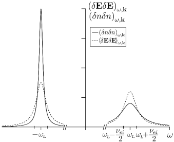
Figure 1: The electron form factor $(\delta n_{e}\delta n_{e})_{\omega,\mathbf{k}}$ ( solid line) and the spectral function of electrostatic field fluctuations $(\delta\mathbf{E}\delta\mathbf{E})_{\omega,\mathbf{k}}$ (dashed line) as a function of frequency. $\mathbf{k\cdot}\frac{\partial n}{\partial\mathbf{r}}=\frac{\nu_{ei}nk_{D}^{2}}{54\omega_{L}};$ $\frac{k_{D}}{k}=6$

References

• [1] J.P. Dougherty and D.T. Farley, Proc. Roy. Soc. A259, 79 (1960); W. Thompson and J. Hubbard, Rev. Mod. Phys. 32, 716 (1960); J. Sheffield, Plasma Scattering of Electromagnetic Radiation (Academic Press, New York, 1975); A. Akhiezer, I. Akhiezer, R. Polovin, A. Sitenko, and K. Stepanov, Plasma Electrodynamics, Vol.1, Linear Theory (Pergamon, Oxford,1975).
• [2] H.B. Callen and T.A. Welton, Phys. Rev. 83, 34 (1951).
• [3] V.V. Belyi and I. Paiva-Veretennicoff, J. of Plasma Physics 43, 1 (1990).
• [4] Yu.L. Klimontovich, Kinetic Theory for Nonideal Gases and Nonideal Plasma (Academic Press, New York, 1975).
• [5] V.V. Belyi Phys. Rev. Lett. 88, 255001 (2002)
• [6] V.V. Belyi, Yu.A. Kukharenko, and J. Wallenborn, Phys. Rev. Lett. 76, 3554 (1996); V.V. Belyi, Yu.A. Kukharenko, and J. Wallenborn J. Plasma Physics 59, 657 (1998).
• [7] V.V. Belyi, Yu.A. Kukharenko, and J. Wallenborn, Contrib. Plasma Phys. 42, 3 (2002).
• [8] B.B. Kadomtsev, Plasma Turbulence, Academic, New York, 1965.
• [9] A.A. Rukhadze, V.P. Silin, Sov. Phys.-Usp. 4, 459 (1961).
• [10] Yu.A. Kravtsov and Yu.I. Orlov, Geometrical Optics of Inhomogeneous Media (Springer, Berlin, 1990); M. Bornatici and Yu.A. Kravtsov, Plasma Phys. Control. Fusion 42, 255 (2000).
Refer to caption