Semiclassical ionization dynamics of the hydrogen molecular ion in an electric field of arbitrary orientation

Abstract

Quasi-static models of barrier suppression have played a major role in our understanding of the ionization of atoms and molecules in strong laser fields. Despite their success, in the case of diatomic molecules these studies have so far been restricted to fields aligned with the molecular axis. In this paper we investigate the locations and heights of the potential barriers in the hydrogen molecular ion in an electric field of arbitrary orientation. We find that the barriers undergo bifurcations as the external field strength and direction are varied. This phenomenon represents an unexpected level of intricacy even on this most elementary level of the dynamics. We describe the dynamics of tunnelling ionization through the barriers semiclassically and use our results to shed new light on the success of a recent theory of molecular tunnelling ionization as well as earlier theories that restrict the electric field to be aligned with the molecular axis.

1 Introduction

The description of the electronic dynamics in the hydrogen molecular ion was one of the important issues in the early days of quantum mechanics and was fundamental to the development of quantum chemistry [1, 2]. Recent progress in different fields of physics has thrust this seemingly museumish, if venerable problem back into the focus of current research: the study of the nonlinear, nonperturbative interaction of matter with intense, ultrashort pulses [3, 4, 5] and of the fascinating internal dynamics of Rydberg plasmas [6, 7, 8, 9]. Both demand the investigation of the electron motion under the influence of two stationary Coulomb centres (TCC) and an external static electric field: On the one hand, quasistatic models of laser-matter interaction that neglect the time-dependence of the laser field have here been surprisingly successful [10, 11, 12, 5]. On the other hand, in a cold plasma the background ions are almost stationary, so that their Coulomb fields are static to a good approximation [13].

In the present paper, we initiate an investigation of the classical and semiclassical mechanics of the electron motion under the influence of two Coulomb centres and an external field of arbitrary orientation. We focus on a description of the saddle points of the relevant potential because they regulate the ionization of the molecule [14]. The locations and heights of the saddles depend on the orientation of the external field and on its strength. Apart from this expected smooth change, we find bifurcation points where additional potential saddles are created or collide and are destroyed. The occurrence of bifurcations even on this most elementary level of the dynamics indicates that the full dynamics must be much more intricate than appears at first sight. The heights of the potential saddles determine the possibility or impossibility of classical over-the-barrier ionization. They depend strongly on the direction of the field. After a detailed discussion of the onset of over-the-barrier ionization, we turn the dynamics of tunnelling ionization, which has recently been the subject of intense study [15, 16, 17]. Using methods of modern nonlinear dynamics, we propose a dynamical mechanism that underlies the success of recent theory of molecular tunnelling ionization [17] that is fashioned after the well-known Ammosov-Delone-Kraĭnov (ADK) theory [18]. The techniques we apply are based on classical mechanics that obeys scaling laws (see section 2). For this reason, although we focus our exposition on the laser ionization of molecules, the results are equally valid for the much larger internuclear distances relevant to the physics of Rydberg plasmas. At the same time, our methods generalize straightforwardly to more complicated systems, such as the electronic motion under the influence of more than two Coulomb centres, possibly in the presence of electric and magnetic fields.

In contrast to atoms, which are spherically symmetric in the absence of external fields, a diatomic molecule possesses a preferred molecular axis. The reaction of the molecule to an electric field will depend not only on the field strength, but also on its direction. In addition, an atom in an external field retains rotational symmetry around the field axis, which renders the electronic dynamics effectively two-dimensional. In a molecule any external field that is not aligned with the molecular axis breaks all continuous symmetries, leads to a strong coupling of all three degrees of freedom and thus induces a significantly more complicated dynamics. Because it has been shown both experimentally [19, 20] and theoretically [21, 22] that a diatomic molecule in a strong laser field experiences a torque that tends to align its axis with that of the electric field, and also because it avoids the intricacies due to the inclusion of an additional degree of freedom, investigations of the quasistatic dynamics have mainly been restricted to the two-dimensional case of parallel axes [23, 24, 25, 26, 27, 28]. In many cases, the ionization of the molecule was even described in terms of a one-dimensional model [23, 24, 25]. However, first investigations of the misaligned case [29] show that its dynamics is remarkably different from the case of aligned axes.

Classical and semiclassical methods such as the field ionization–Coulomb explosion (FICE) model [23, 24, 25] have served well to illuminate the dynamics of molecular ionization in a static field. Their virtue is that they can provide an intuitive picture of the essential dynamics, even in situations where many coupled degrees of freedom are involved and that are intractable by exact quantum mechanical methods. For this reason it is highly desirable to make their power available to the description of the general case which, due to the complete breaking of symmetries, can be expected to be much more complex. In this paper, we will embark on a description of the electronic dynamics in the field of two stationary Coulomb centres (TCC) together with a static electric field of arbitrary strength and arbitrary orientation. Given the success of the FICE model [23, 24, 25] for the collinear configuration of non-hydrogenic and even heteronuclear molecules, we expect our results to be valuable beyond the hydrogen molecular ion for a wide range of more complicated molecules.

We will focus on the description of the saddle points of the TCC system in an electric field, i.e. the unstable equilibrium points where the electron can be at rest. They are the critical bottlenecks where ionization takes place. It has been shown recently [14] that, using the methods of modern nonlinear dynamics, one can compute ionization rates of atoms in external fields from a detailed description of the saddle points. Therefore, after laying out some general properties of the TCC potential in an external field in section 2, we will, in section 3, start our investigation with the identification of the saddle points the potential possesses. Already in this seemingly elementary first step, we will encounter the richness the dynamics of our system exhibits: We will find that the potential saddles undergo bifurcations as the field strength and field direction are varied, so that for any given external field either two or four saddle points can coexist. We will also see that the saddles differ in their indicess, i.e. in the number of unstable directions attached to them.

The most fundamental property of a saddle point is its height. The height determines if classical over-the-barrier ionization can take place (namely, when the saddle is lower than the electron energy) or is forbidden. It therefore marks the onset of ionization. We will discuss the heights of the different saddles as function of field strength, field direction and internuclear distance in section 4.

If the energy of a bound electron is lower than the classical ionization threshold, the molecule can still ionize by means of tunnelling [30, 31, 10]. This process is commonly described by the ADK model [18], which uses the ionization rate of a hydrogen atom or hydrogen-like ion in a static external field. In that system, ionization takes place predominantly along the axis of the external electric field, so that the description of the ionization process reduces to a one-dimensional tunnelling calculation. The ADK model has recently been generalized by Tong et al[17] to explain the tunnelling ionization of diatomic molecules. These authors explain the ionization suppression found experimentally for a wide range of molecules by taking into account the anisotropy of the bound-state molecular wave functions. They neglect, however, the coupling of the different degrees of freedom that is absent in atomic ionization, but relevant in a molecule. In section 5 we will analyze the tunnelling dynamics for the hydrogen molecular ion in a misaligned electric field from the point of view of nonlinear dynamics and thereby elucidate the reason why the approach of Tong et alcould nevertheless succeed. Our approach will also clarify the success of theories that assume the electric field to be aligned with the molecular axis [23, 15, 24, 25, 26, 27].

2 The TCC potential in an electric field

In the following, we will discuss the dynamics of an electron under the combined influence of two stationary nuclei of charge $Z$ and a homogeneous static electric field. We will choose the coordinate system so that the external field is in the $xz$-plane and the nuclei are lying on the $z$-axis, at a distance $c$ on both sides of the origin. With these conventions, the electronic dynamics can be described by the Hamiltonian, in atomic units,

$$H=\frac{{\bi p}^{2}}{2}+V({\bi x})$$ (1)

with the potential

$$V({\bi x})=-\frac{Z}{\left(x^{2}+y^{2}+(z-c)^{2}\right)^{1/2}}-\frac{Z}{\left(x^{2}+y^{2}+(z+c)^{2}\right)^{1/2}}-Fz\cos\phi-Fx\sin\phi\;.$$ (2)

Here, $F$ is the strength of the external field. The angle $\phi$ between the field and the negative $z$-axis uniquely specifies the field direction. Notice that we have taken $V$ to denote the potential energy of an electron with negative unit charge. It is the negative of the electrostatic potential.

Apart from the external field strength and direction, the potential (2) and the Hamiltonian (1) depend on the nuclear charge $Z$ and the internuclear distance $2c$. Those dependences can be removed by introducing the scaled quantities

$$\tilde{\bi x}={\bi x}/c\;,\qquad\tilde{\bi p}=(c/Z)^{1/2}{\bi p}\;,$$

$$\tilde{F}=c^{2}F/Z\;,$$

$$\tilde{H}=cH/Z\;,\qquad\tilde{V}=cV/Z\;.$$ (3)

In terms of these scaled variables, the scaled Hamiltonian reads

$$\tilde{H}=\frac{\tilde{\bi p}^{2}}{2}+\tilde{V}(\tilde{\bi x})$$ (4)

with the scaled potential

$$\tilde{V}(\tilde{\bi x})=-\frac{1}{\left(\tilde{x}^{2}+\tilde{y}^{2}+(\tilde{z}-1)^{2}\right)^{1/2}}-\frac{1}{\left(\tilde{x}^{2}+\tilde{y}^{2}+(\tilde{z}+1)^{2}\right)^{1/2}}-\tilde{F}\tilde{z}\cos\phi-\tilde{F}\tilde{x}\sin\phi\;.$$ (5)

The nuclear charges have been scaled to 1 and the internuclear distance to 2. It is this scaled form of the dynamics that we will use in most of what follows, returning to the unscaled variables as necessary.

Notice that the Hamiltonian (4) is symmetric with respect to a reflection in the $xz$-plane, so that this plane is invariant under the dynamics. Furthermore, for $\phi=90^{\circ}$ the external field is oriented along the $x$-axis and there is an additional symmetry with respect to reflection in the $xy$-plane. In the general case, a reflection in that plane takes an external field oriented at an angle $\phi$ from the negative $z$-axis into a field oriented at an angle $180^{\circ}-\phi$, so that the dynamics in these two situations agree.

3 The potential saddles of the TCC system in an electric field

In this section we will identify and describe the equilibrium points of the potential (5) where $\nabla\tilde{V}=0$. Section 3.1 describes their locations. In a second step, in section 3.2, we will compute the Hessian matrix of the potential in these points to classify them as potential maxima, minima or saddles.

3.1 The location of equilibria

The task of finding the stationary points of the combined potential can be rephrased as finding those points where the Coulomb field caused by the two centres is equal in magnitude and opposite in direction to the applied external field. We will therefore, in this section, restrict ourselves to a discussion of the pure TCC potential and locate those points where the TCC electric field has a given strength and direction. For symmetry reasons it is obvious that these points can only lie in the $xz$-plane spanned by the molecular axis and the direction of the external field. We can therefore further restrict our discussion to the TCC field strength in that plane. Due to the sign conventions taken in (2), the external field makes an angle $\phi$ with the negative $z$-axis and, if $\phi$ is chosen in the interval $0<\phi<180^{\circ}$, has a negative $x$ component. As a consequence, the TCC field balancing the external field must have a positive $x$ component and make and angle $\phi$ with the positive $z$-axis. This is the range of parameters to which we will restrict our attention in the following.

Figure 1: (a) Contour lines of the absolute value of the TCC electric field strength. (b) Contour lines of the angle $\phi$ between the TCC electric field and the positive $\tilde{z}$-axis. Thick lines: 90-degree angle line, thin solid lines: angle lines $\phi<90^{\circ}$, dashed lines: $\phi>90^{\circ}$.

Let us first discuss the absolute value of the TCC field strength, disregarding the field direction. The variation of field strength in the $xz$-plane is illustrated in figure 1(a). Regions of high field strength are located in the vicinity of either nucleus. There, the field caused by the close-by nucleus is much stronger than that of the remote nucleus, so that the lines of constant field strength are nearly concentric circles around the nucleus. At the other extreme, the field strength is zero at the midpoint between the nuclei, i.e. at $x=z=0$, as well as infinitely far from the centres. For sufficiently low field strengths, therefore, there is a field strength line surrounding the midpoint and a second strength line surrounding both centres.

Thus, although the topology of field strength lines is different for high and for low field strength, for any given field strength there are two disjoint contours. The transition between the different topologies occurs for the critical field strength $\tilde{F}_{\rm c}$ where the disjoint contours merge and intersect at right angles. It can be inferred from figure 1(a) that $\tilde{F}_{\rm c}$ is the maximum field strength taken on the $x$-axis. From this observation we can calculate that $\tilde{F}_{\rm c}=4/(3\sqrt{3})=0.7698$.

We now turn to a description of the direction of the two-centre Coulomb field, which is illustrated in figure 1(b). We first look for those locations where the field is perpendicular to the molecular axis. Due to symmetry, it is clear that this is the case on the $\tilde{x}$-axis. In addition, 90-degree angle lines emanate from either nucleus and join the $\tilde{x}$-axis at $\tilde{x}=\sqrt{2}$. As can be seen from figure 1(b), they partition each quadrant of the $\tilde{x}\tilde{z}$-plane into an “inner” region close to $\tilde{x}=\tilde{z}=0$ and an “outer” region at large $\tilde{x}$ and $\tilde{z}$. The angle lines for angles $\phi<90^{\circ}$ fill the outer region of the quadrant $\tilde{z}>0$ and the inner region of the quadrant $\tilde{z}<0$. Symmetrically, the angle lines for $\phi>90^{\circ}$ fill the inner region of the quadrant $\tilde{z}>0$ and the outer region of the quadrant $\tilde{z}<0$. Thus, any angle line for $\phi\neq 90^{\circ}$ has two disjoint parts. The 90-degree angle lines themselves correspond to the critical value where the two parts of the angle lines connect and change their topology.

Comparing figures 1(b) and 1(a), it becomes clear that as we follow the outer part of any angle line from the nucleus out to infinity, the field strength will decrease monotonically from infinity to zero. As a consequence, any field strength is assumed exactly once. If we apply an arbitrary external field, we will find a unique equilibrium point on the corresponding outer angle line where the Coulomb field exactly cancels the external field. We call it the outer saddle point.

On the inner angle lines, the situation is more complicated. For sufficiently small field angles $\phi$, the field strength along the inner angle line will increase monotonically from zero to infinity as the line is followed from midpoint to the nucleus. Therefore, in this case we will find a single equilibrium on the inner angle line that will turn out to be an inner saddle point.

Figure 2: TCC field strengths measured along the inner angle lines for field angles (a) $\phi=75^{\circ}$, (b) $\phi=\phi_{\rm min}=81.6014^{\circ}$, (c) $\phi=86^{\circ}$. The parameter $\tilde{L}$ is the arc length of the angle line, measured from the midpoint between the nuclei.

Figure 3: Minimum and maximum scaled field strengths $\tilde{F}_{\rm min}(\phi)$ and $\tilde{F}_{\rm max}(\phi)$ bounding the parameter region where three inner equilibria exist.

For field angles $\phi$ close to $90^{\circ}$, however, the field strength along the inner angle line approximates the field strength along the 90-degree line. It rises from zero at the midpoint to a maximum $\tilde{F}_{\rm max}(\phi)\approx\tilde{F}_{\rm c}$, then decreases to a minimum $\tilde{F}_{\rm min}(\phi)$ and finally increases to infinity at the nucleus. This behaviour is illustrated in figure 2. It is found for angles in the interval $\phi_{\rm min}<\phi<\phi_{\rm max}$, where $\phi_{\rm min}=81.6014^{\circ}$ and $\phi_{\rm max}=180^{\circ}-\phi_{\rm min}=98.3986^{\circ}$. As a consequence, if the field angle is chosen in this interval, there is a unique inner equilibrium if the field strength is outside the interval $\tilde{F}_{\rm min}(\phi)<\tilde{F}<\tilde{F}_{\rm max}(\phi)$, but there are three inner equilibria if the field strength is within that interval. The domain of field strengths and field angles where multiple inner equilibria occur is depicted in figure 3.

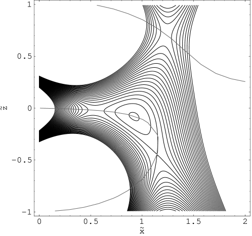
Figure 4: Contour plot of the total potential for the TCC system in an external electric field for a configuration with three inner equilibria. The scaled field strength is $\tilde{F}=0.74$, the angle with the molecular axis $\phi=87^{\circ}$. The $87^{\circ}$-angle lines are indicated for clarity.

For a field configuration where three inner equilibria exist, the potential in the $\tilde{x}\tilde{z}$-plane is shown in figure 4. It exhibits a saddle, a maximum, and a saddle along the inner angle line. As the external field is varied and leaves the region of multiple equilibria in figure 3, bifurcations of the equilibria must occur. Specifically, as the upper critical field strength $\tilde{F}_{\rm max}$ is approached from below, the maximum will collide with the saddle to its left in the figure and they will annihilate, forming what in the language of Catastrophe Theory [32, 33] is called a “fold” catastrophe. Similarly, as the lower critical field strength $\tilde{F}_{\rm min}$ is approached, the maximum will collide and annihilate with the saddle below in the figure.

The most degenerate field configuration arises for the extremal angles $\phi_{\rm min}$ and $\phi_{\rm max}$ where the lower and upper critical field strengths coincide. For these parameter values, all three inner equilibria coalesce. If we follow the potential along the angle line in this situation, we find a minimum of fourth order. In the parlance of Catastrophe Theory, this scenario is called a “cusp” catastrophe. It also occurs for $\phi=90^{\circ}$ if the field strength is chosen such that the saddles on the two outer 90-degree lines approach the $\tilde{x}$-axis and there coalesce with a maximum on that axis. This bifurcation forms the lower corner of the “triangle” in figure 3 that bounds the region of three inner equilibria. In all three corners of that triangle, its edges meet tangentially, as is predicted by the theory of the cusp catastrophe [32, 33].

3.2 The classification of equilibria

Once we have found the equilibria of the TCC system in an external electric field, which we have achieved in section 3.1, we must classify them according to the number of unstable degrees of freedom the dynamics possesses in their neighbourhood. That number is given by the number of negative eigenvalues of the Hessian determinant. We call it the index of the equilibrium point [33]. Note that it suffices to discuss the behaviour of the potential in the $\tilde{x}\tilde{z}$-plane of the three-dimensional potential. The motion in the $\tilde{y}$ degree of freedom decouples from the dynamics in the symmetry plane in the harmonic approximation and is always stable: As we move away from the plane, the distances to both nuclei increase and the potential goes up. Thus, an equilibrium that is found to be a potential saddle in the plane is a saddle of index one of the three-dimensional potential. Similarly, a maximum of the planar potential corresponds to a saddle of index two and a minimum of the planar potential to a minimum (with index zero) of the three-dimensional potential.

To classify the equilibria of the planar potential, note that the (scaled) planar Hessian determinant

$${\rm Hess}(\tilde{x},\tilde{z})=\det\left(\begin{array}[]{cc}\frac{\partial^{2}\tilde{V}}{\partial^{2}\tilde{x}}&\frac{\partial^{2}\tilde{V}}{\partial\tilde{x}\partial\tilde{z}}\\ \frac{\partial^{2}\tilde{V}}{\partial\tilde{z}\partial\tilde{x}}&\frac{\partial^{2}\tilde{V}}{\partial^{2}\tilde{z}}\end{array}\right)$$ (6)

of the potential $\tilde{V}$ is negative at a saddle and positive at a maximum or minimum. Furthermore, since the second derivatives of the linear external potential are zero, we can evaluate the Hessian of the TCC potential instead of the total potential.

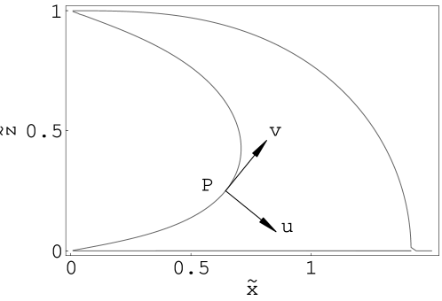
Figure 5: The coordinate system used for the calculation of the Hessian determinant. See text for a description.

To compute the Hessian at a point $P$, we introduce a Cartesian coordinate system $(u,v)$ such that the $v$-axis is tangential to the angle line through $P$ (see figure 5). Using the fact that the TCC electric electric field strength $\tilde{\bi F}_{\rm TCC}=\nabla\tilde{V}_{\rm TCC}$, we can rewrite the Hessian (6) as

$${\rm Hess}(P)=\det\left(\begin{array}[]{cc}\frac{\partial F_{u}}{\partial u}&\frac{\partial F_{u}}{\partial v}\\ \frac{\partial F_{v}}{\partial u}&\frac{\partial F_{v}}{\partial v}\end{array}\right)\;,$$ (7)

where

$$F_{u}=\tilde{F}\sin\psi\;,\qquad F_{v}=\tilde{F}\cos\psi$$ (8)

are the $u$ and $v$ components of the scaled TCC electric field strength and $\psi$ is the angle between the electric field and the positive $v$-axis. If $\alpha$ denotes the angle between the $v$- and $\tilde{z}$-axes, $\psi$ is given by $\psi=\phi-\alpha$. Due to our choice of the $v$-axis along the angle line, we have

$$\left.\frac{\partial\psi}{\partial v}\right|_{P}=0\;,$$

so that the Hessian (7) with (8) simplifies to

$${\rm Hess}(P)=\tilde{F}\,\frac{\partial\tilde{F}}{\partial v}\,\frac{\partial\psi}{\partial u}=\tilde{F}\,\frac{\partial\tilde{F}}{\partial v}\,\frac{\partial\phi}{\partial u}\;.$$ (9)

Referring back to figure 1(b), we see that in the inner region shown $\partial\phi/\partial u$ is negative, because the $u$-axis points from an angle line $\phi>90^{\circ}$ toward the 90-degree line. We thus obtain the result that the Hessian of the potential at an equilibrium point $P$ is negative, i.e. $P$ is a saddle point, if and only if the derivative of the field strength along the angle line is positive. That field strength has already been discussed above. It is illustrated in figure 2. (The orientation of the angle line chosen there is the same as the orientation of the $v$-axis in figure 5.) The field strength is monotonically increasing along the angle line whenever there is a single inner equilibrium, which therefore is a saddle. For angles and field strengths where three inner equilibria exist, the first and the third encountered along the angle line are in a region of increasing field strength and are therefore saddles, whereas the second is either a maximum or a minimum of the potential. As long as the angle between the positive $v$-axis and the Coulomb field is less then $90^{\circ}$, which is certainly the case in the part of the angle line that closely follows the $\tilde{x}$-axis, one can further show that the potential has a maximum along the angle line if $\partial\tilde{F}/\partial v<0$. Thus, the second equilibrium is found to be a maximum. By a similar argument, it can be shown that the index of the outer saddle is always one.

4 Classical ionization thresholds

Having found the locations of the saddle points of the TCC potential in an electric field, we now turn to a discussion of their heights, which ultimately determine the possibility of classical over-the-barrier ionization. We will focus, in particular, on the dependence of the barrier heights upon the field angle. Before a discussion of general field orientations, it will be useful to consider the extremal cases where the electric field is oriented either parallel or perpendicular to the molecular axis.

4.1 Barriers in a perpendicular field

The perpendicular field configuration is special in that in addition to the reflection symmetry in the $xz$-plane there is another symmetry with respect to the $xy$-plane perpendicular to the molecular axis. As a consequence, saddle points must either lie in that plane (i.e. on the $x$-axis) or occur in symmetrical pairs.

Figure 6: The heights of the potential saddles as a function of the electric field strength for $\phi=90^{\circ}$. Solid line: outer saddle, long-dashed line: inner saddle, short-dashed line: saddle of index two. All of these saddles are located on the $x$-axis. Dash-dotted line: symmetric pair of saddles away from the $x$-axis. The inset shows an enlarged view of the bifurcation region.

If the scaled field strength is low, there are an inner and an outer saddle on the $x$-axis. With increasing field strength, the inner saddle moves outward and the outer saddle inward. At $\tilde{F}=\tilde{F}_{1}=(2/3)^{3/2}=0.5443$ the outer saddle crosses the point $\tilde{x}=\sqrt{2}$ where the outer 90-degree angle lines reach the $x$-axis. At this point, it turns into a saddle of index two, and a symmetric pair of saddles of index one on the outer 90-degree lines is born. As the field strength increases further, the latter move toward the nuclei along the angle lines. The saddle of index two collides and annihilates with the inner saddle at $\tilde{F}=\tilde{F}_{2}=4/(3\sqrt{3})=0.7698$. This leaves only the pair of symmetric saddles at high field strength. Because the 90-degree lines form the boundary between inner and outer angle lines, these saddles can at will be classified as either “inner” or “outer” saddles. Figure 6 illustrates this sequence of events. It also shows that for most field strengths the inner saddle is lower that the outer saddle. As in the case of an axial field [23, 24, 25, 27], the inner saddle allows the electron to switch from one nucleus to the other, not to ionize. Thus, the onset of above-threshold ionization is, as in the axial configuration, determined by the height of the outer saddle.

4.2 Angle-dependence of the barrier heights

Figure 7: The heights of the potential saddles as a function of the field angle $\phi$ for field strengths (a) $\tilde{F}=0.5$, (b) $\tilde{F}=0.75$, (c) $\tilde{F}=0.9$. Solid lines: outer saddle, long-dashed lines: inner saddles of index one, short-dashed lines: saddles of index two. In (b), the inset shows a blow-up view of the bifurcation region.

For arbitrary field angles $\phi$, the heights of the saddle points interpolate between the two extremal cases we have just discussed. Their angle dependence is displayed in figure 7 for three different values of the scaled field strength. The most significant feature the heights exhibit is that for all field strengths the height of the outer saddle increases as the field angle increases from zero to $90^{\circ}$, whereas the height of the inner saddle decreases. Since we have seen in section 4.1 that it is the outer saddle that is most relevant for ionization, it follows that the molecule is easiest to ionize in the parallel configuration and that ionization gets harder the larger an angle the external field makes with the molecular axis.

In accordance with what can be seen in figure 6, the behaviour of the saddle heights in the vicinity of $\phi=90^{\circ}$ is completely different for high and for low field strengths. At low field strength $\tilde{F}<\tilde{F}_{1}$, as in figure 7(a), an inner and an outer saddle exist which are non-degenerate. If the field strength is increased beyond $\phi=90^{\circ}$, the saddle heights symmetrically retrace their paths to reach their values at $\phi=0^{\circ}$ again at $\phi=180^{\circ}$. For this reason, they must have zero slope at $\phi=90^{\circ}$.

For high field strengths $\tilde{F}>\tilde{F}_{2}$, as in figure 7(c), the two saddles are degenerate at $\phi=90^{\circ}$. As the angles increase beyond $90^{\circ}$, the saddles change their roles, the saddle that was “outer” for $\phi<90^{\circ}$ being “inner” for $\phi>90^{\circ}$ and vice versa. It is therefore possible for the heights of these saddles to intersect at $\phi=90^{\circ}$ with non-zero slope. In the intermediate field strength regime $\tilde{F}_{1}<\tilde{F}<\tilde{F}_{2}$, which is illustrated in figure 7(b), both types of behaviour can be observed at the same time.

4.3 Barrier heights as a function of the internuclear distance

Figure 8: Unscaled barrier heights as a function of the internuclear separation $R$ for fixed external electric field strength $F=0.053\,38\,{\rm a.u.}$, nuclear charge $Z=1$ and field angles (a) $\phi=50^{\circ}$, (b) $\phi=85^{\circ}$. Solid lines: outer saddle, dashed lines: inner saddles. Dash-dotted lines mark the asymptotic barrier heights (11) for large $R$.

So far, we have described the potential saddles as a function of the direction and the scaled strength of the external electric field. While this procedure facilitates the structural understanding of the saddles and their bifurcations, it is somewhat remote from experimental conditions where an external field of a certain non-scaled strength is given and the value of the scaled field strength depends on the separation of the nuclei. It can thus change considerably in time if the molecule dissociates under the influence of the field. To approach this situation, we now turn to a discussion of the saddle heights as a function of the internuclear distance $R$ for fixed external field strength $F$. Results are shown in figure 8 for $F=0.053\,38\,{\rm a.u.}$, which is the peak field strength of a linearly polarized laser field with an intensity of $10^{14}\,{\rm W\,cm^{-2}}$. The nuclear charge was chosen to be $Z=1$, as is appropriate for a hydrogen molecular ion.

The most conspicuous feature of figure 8 is that the height of the inner saddle diverges to $-\infty$ for $R\to 0$ whereas the height of the outer saddle remains finite. This behaviour can be understood by noting that the limit $R\to 0$ corresponds to the united-atom limit where the two nuclei coincide to form a single nucleus of double charge. If a hydrogen-like atom of nuclear charge $z$ is exposed to an external electric field of strength $F$, there is a single potential “Stark”-saddle whose height is [34]

$$V_{\rm Stark}=-2\sqrt{zF}\;.$$ (10)

For the field strength used in figure 8, the Stark saddle height is $V_{\rm Stark}=0.6535\,{\rm a.u.}$, which is the value approached by the outer saddle height. It is independent of the field angle $\phi$ because in the united-atom limit the notion of an intermolecular axis becomes meaningless. The inner saddle, by contrast, is always located within a few $R$ of either nucleus. Thus, in the limit $R\to 0$ it approaches both nuclei, so that the saddle height must diverge.

In the opposite limit of large internuclear distance, the nuclei are so far apart that their Coulomb wells barely overlap. Therefore, if an external field is present, to each nucleus there is attached a Stark saddle point whose height relative to the value of the external potential at the location of the nucleus is given by (10). The nuclei themselves are displaced to opposite sides from the zero of the external potential, which we have chosen in (2) to be at the midpoint between the nuclei. The total height of the two saddles in the separated-atom limit is thus

$$V_{\rm sep}=-2\sqrt{F}\pm\frac{R}{2}F\cos\phi\;.$$ (11)

These asymptotic saddle heights are indicated by the dash-dotted lines in figure 8. From figure 1(b) it becomes clear that the inner saddle is shifted into the direction of higher external potential, the outer saddle into the direction of lower potential. Thus, the inner saddle height must approach the higher of the two asymptotic values (11) while the outer saddle height approaches the lower value.

Due to the asymptotic behaviour (11), the height of the inner saddle increases with $R$ for large internuclear distances, the height of the lower saddle decreases. However, the distance-dependence of the asymptotic heights (11) becomes slight when the angle approaches $90^{\circ}$, so that the asymptotic behaviour sets in only for very large distances. Thus, for large angles we find that the outer barrier height is actually increasing with the internuclear separation over the physically relevant range of distances.

Figure 9: Enlarged detail of figure 8(c), showing the bifurcations of the inner saddles. Long-dashed lines: saddles of index one, short-dashed line: saddle of index two.

At first sight, the bifurcations of the inner saddles seem to have no impact whatsoever on the behaviour of the barrier heights in figure 8. Upon a closer look, however, one discovers a little “knee” in the inner saddle height for $\phi=85^{\circ}$ at $R\approx 7.5\,{\rm a.u}$. At this point the curve seems to change its slope discontinuously. If we enlarge this part of the curve, as shown in figure 9, we find that this is indeed the region where the bifurcations take place. In a small range of internuclear distances, a new saddle of index one is created and the previously-existing saddle is destroyed. This shift from one saddle to the other gives rise to the apparently discontinuous bend observed in figure 8(b).

5 Tunnelling ionization

Even if the electron energy is below the barrier height discussed in section 4, ionization can still take place due to quantum mechanical tunnelling. In atoms, this process is commonly described in the framework of the ADK model [18], which uses the ionization rate of a hydrogen atom or a hydrogen-like ion in a static external field. In that system, ionization takes place predominantly along the axis of the external electric field, so that the description of the ionization process reduces to an essentially one-dimensional tunnelling calculation which matches the wave function within the well to the ionizing parts of the wave function beyond the barrier. To generalize this approach to the ionization of molecules, a double modification is necessary: On the one hand, a molecular wave function is anisotropic, so that the ionization rate will depend on the direction in which ionization is taking place, i.e. on the direction of the external field. On the other hand, in the complicated potential (2), unlike for the hydrogen atom in an electric field [34, 35], the different degrees of freedom do not decouple, so that the tunnelling process cannot be regarded as essentially one-dimensional. This coupling of the different degrees of freedom must also be taken into account.

Recently, Tong et al[17] proposed a generalization of the ADK model of tunnelling ionization to the ionization of diatomic molecules. They take into account the anisotropy of the bound-state molecular wave function, but they retain an essentially one-dimensional picture of the tunnelling process and fail to discuss the impact of multiple coupled degrees of freedom. We will here analyze the tunnelling paths for the hydrogen molecular ion in a non-axial electric field and thereby elucidate the reason why the quasi one-dimensional approach of Tong et alcould succeed even though the effects of the additional degrees of freedom were neglected.

Different approaches to the theory of barrier-suppression ionization are surveyed by Kraĭnov [36]. We will here adopt a semiclassical description of the ionization process. Within that framework, the tunnelling transmission probability through a barrier [37]

$$P=\frac{1}{1+\rme^{K/\hbar}}$$ (12)

is determined by the action integral

$$K=\int|p|\,dq$$ (13)

along the tunnelling path, with

$$p({\bi x})=\sqrt{2(E-V({\bi x}))}$$ (14)

the (imaginary) momentum the electron has at the position $\bi x$ below the barrier, $V({\bi x})>E$. Kraĭnov [36] gives a formula for the tunnelling probability in the case of a hydrogen atom in an electric field that is obtained from (12) if the barrier is assumed parabolic. In its more general form, equation (12) is applicable to parabolic as well as non-parabolic barriers and in one as well as several degrees of freedom. In one dimension, the action (13) is computed along the unique path leading from one side of the barrier to the other. In several dimensions, however, an infinity of possible tunnelling paths connect the region of bound motion at a given energy to the region of free motion, and it is not obvious along what path the tunnelling action (13) should be taken. A similar difficulty arises if the strictly quantum mechanical method of the phase functions [36] is used in multiple degrees of freedom. Thus, we expect the results described below to be valuable beyond the limits of the semiclassical theory.

If reactant and product regions of configuration space are separated by a saddle point in a multidimensional potential, the path of steepest descent from the saddle is regarded as the “reaction path” in chemistry (see, e.g., [38]). However, it is also well known that the tunnelling integral taken along that path can severely underestimate the extent of tunnelling. To obtain the transmission probability correctly, the path must be chosen such as to maximize (12), i.e. to minimize the tunnelling action (13). In cases where the reaction path is strongly curved, the tunnelling path lies on its concave side (“corner cutting”) [39], which shortens the path and helps minimize the tunnelling action.

Through (14) the optimum tunnelling path depends crucially on the details of the potential, or equivalently the dynamics, in the vicinity of the saddle point. To analyze it, it is helpful to allow coordinates, momenta and the time to assume complex rather than real values. This artifice allows us extend the classical dynamics to the region below the barrier and makes the full machinery of classical dynamics available to an analysis of the tunnelling process. If we do so, by virtue of Maupertuis’ principle [35] the requirement to minimize the tunnelling action (13) translates into the condition that the tunnelling path be the configuration space projection of a classical trajectory. In addition, the tunnelling path must start and end on the energy contour $V({\bi x})=E$, where the real dynamics can take over. At these points, it must have zero momentum. Using the time-reversal invariance of the dynamics described by the Hamiltonian (1), we can conclude that the tunnelling orbit must be periodic. This leads us to the prescription to identify the optimum tunnelling path as the configuration space projection of an imaginary-time complex periodic orbit under the potential barrier. Equivalently, it can be found as the projection of a real periodic orbit in the inverted potential [40].

Figure 10: Optimum tunnelling paths for tunnelling under the outer (left column) and inner (right column) saddles at different energies for a scaled external electric field strength of $\tilde{F}=0.5$ and field angles (a) $\phi=30^{\circ}$, (b) $\phi=60^{\circ}$, and (c) $\phi=80^{\circ}$.

Using the above prescription, we can compute the tunnelling paths for arbitrary external field strengths, field directions and tunnelling energies. Results for a scaled external field strength $\tilde{F}=0.5$ are shown in figure 10. These tunnelling paths show the expected shift to the concave side of the reaction path, but the amount of corner cutting is small because, especially for small angles and for the outer saddle, the reaction path is close to a straight line. This is a clear indication of quasi one-dimensional tunnelling dynamics.

Figure 11: Tunnelling actions for scaled electric field strength $\tilde{F}=0.5$ and different field angles, plotted as a function of absolute scaled energy (a) and scaled energy difference below the height of the saddle point (b).

Even more striking is the behaviour of the tunnelling actions shown in figure 11. The curves in figure 11(a) present the energy-dependence of the tunnelling action below the outer saddle for different angles. They differ mainly in the height of the saddle point in which they originate. This is especially clear when all energies are referred to the respective saddle point energies, as in figure 11(b). In this case, all action curves nearly coincide. An exception is formed by the curve for $\phi=90^{\circ}$. This curve is lying on the $x$-axis, as are both saddle points. If the energy is below the height of the inner saddle, the periodic tunnelling orbit will cross that saddle and the tunnelling path described above will cease to exist. The presence of the second saddle distorts the action curve away from the universal behaviour of the other curves and finally causes it to end.

The nearly universal tunnelling dynamics is due to the fact that the outer saddle, especially for small field angles, is much closer to one of the nuclei than to the other. Thus, the neighbourhood of the saddle is very similar to that of the Stark saddle encountered in a single atom in an electric field. The tunnelling dynamics is therefore similar the atomic tunnelling dynamics, and the ionization rate is closely approximated by the ADK rate once the distortion of the molecular wave function through the presence of the second nucleus is taken into account. The tunnelling rate will, however, depend on the field angle through the height of the saddle. Very similar results are found for the higher scaled field strength $\tilde{F}=0.75$.

Figure 12: Tunnelling actions for scaled electric field strength $\tilde{F}=0.05338$ and different field angles, plotted as a function of scaled energy.

The universality of the tunnelling dynamics is even more pronounced for the lower scaled field strength $\tilde{F}=0.053\,38$, which is the peak field strength in a linearly polarized laser beam with an intensity of $10^{14}{\rm W\,cm}^{-2}$. In this case, the inner saddle point is very close to the origin $\tilde{x}=\tilde{z}=0$, so that the inner tunnelling paths lie virtually on the $\tilde{z}$-axis. The outer saddle is located at a scaled distance from the origin between 6.35 at $\phi=0$ and 6.00 at $\phi=90^{\circ}$. For these large distances, we approach the united-atom limit, which explains why the angle dependence of the distance is slight. As a further consequence, both the saddle shapes and saddle heights are well approximated by the Stark saddle of the united atom, as is confirmed by the tunnelling actions shown in figure 12. We find not only that the outer saddle height is virtually independent of the field angle, but also that the tunnelling action is a nearly universal function of the tunnelling energy for all angles including $\phi=90^{\circ}$. At this field strength, the inner saddle is sufficiently far away from the outer saddle so that it does not cause any distortion or singularity in the energy range shown.

The experimental data used by Tong et al [17] was taken at laser intensities around $I=10^{14}\,{\rm W\,cm^{-2}}$, which corresponds to a peak field strength of $F=0.053\,38\,{\rm a.u.}$ and, for an internuclear separation of $2\,{\rm a.u.}$, to the scaled field strength of $\tilde{F}\approx 0.053\,38$ we have studied above. It is well within the range of field strengths where the angle-independent behaviour of the united-atom limit holds. For a neutral molecule, in particular a non-hydrogenic molecule as in [17], the effective potential experienced by the ionizing electron is more complicated than the potential (2) due to the presence of the inner electrons. However, these deviations from Coulombic behaviour arise mainly in the vicinity of the nuclei. For the (on an atomic scale) weak fields relevant to [17], the saddle is far away from the nuclei and we can expect the simple potential (2) to approximate the true tunnelling dynamics well.

We can therefore conclude that for small field strengths the effects of reaction path curvature that were not considered by Tong et alhave little impact on the tunnelling ionization of a molecule because the electron is essentially subject to the Coulomb field of the united nuclei. They will become even smaller when averaged over the external field direction. This observation explains why the quasi-atomic tunnelling theory of [17] could succeed without taking these dynamical effects into account. At the same time, the angle-independence of the tunnelling dynamics explains why previous theories of ionization that only deal with the special case of an axial field [23, 15, 24, 25, 26, 27, 28] yield results in resonable agreement with experiment although in an experiment one has no control over the relative orientations of the molecule and the field.

In the opposite limit of strong external field, we regain a similar universal tunnelling dynamics because the saddle points approach individual nuclei and the influence of the remote nucleus becomes small. As we have found only small deviations from universal quasi-atomic dynamics even for intermediate field strength, we can conclude that the effects of reaction path curvature are small for all field strengths.

6 Conclusion

As a first step toward an understanding of the electronic dynamics of the hydrogen molecular ion in an electric field of arbitrary orientation, we have presented a detailed discussion of the saddle points of the relevant potential. We have found that the saddle points bifurcate as the external electric field strength and direction are varied, which gives us a first glimpse of the richness the full dynamics of the system must possess. We used our knowledge of the saddle points to describe both the onset of over-the-barrier ionization and the dynamics of tunnelling ionization below the saddle points, which shed new light on the success of a recent theory of molecular tunnelling ionization [17] as well as previous theories that treat the special case of axial fields [23, 15, 24, 25, 26].

The presentation of the dynamics near the saddle points in the hydrogen molecular ion opens several directions of further investigation: Firstly, it calls for a more thorough investigation of the dynamics within the wells. One can expect to find a wealth of intricate classical structure that could illuminate the finer details of the molecular ionization process, both above and below the classical threshold. Secondly, the connection to quantum mechanics must be established to determine the energies and widths of the bound states within the well in a way analogous to the one-dimensional calculations of [41, 42, 43]. Thirdly, with regard to Rydberg plasmas it is essential to include the Coulomb fields of the surrounding ions and to allow for the presence of a magnetic field. The dynamics of the hydrogen molecular ion in an electric field of arbitrary direction offers a rich and fascinating field of inquiry whose investigation we have here only just begun.

References

References

- [1] Pauli W 1922 Ann. Phys., Lpz 68 177
- [2] Burrau O 1927 Kgl. Danske. Videnskab. Selskab. 7 14
- [3] Bandrauk A D (ed) 1994 Molecules in laser fields (New York: Marcel Dekker)
- [4] Posthumus J (ed) 2001 Molecules and Clusters in Intense Laser Fields (Cambridge, UK: Cambridge University Press)
- [5] Bandrauk A D and Kono H 2003 Advances in Multi-Photon Processes and Spectroscopy vol 15 ed Lin S H, Villaeys A A and Fujimura Y (Singapore: World Scientific) pp 149–214
- [6] Robinson M P, Tolra B L, Noel M W, Gallagher T F and Pillet P 2000 Phys. Rev. Lett. 85 4466
- [7] Dutta S K, Feldbaum D, Walz-Flanigan A, Guest J R and Raithel G 2001 Phys. Rev. Lett. 86 3993
- [8] Killian T C, Kulin S, Bergeson S D, Orozco L A, Orzel C and Rolston S L 1999 Phys. Rev. Lett. 83 4776
- [9] Killian T C, Lim M J, Kulin S, Dumke R, Bergeson S D and Rolston S L 2001 Phys. Rev. Lett. 86 3759
- [10] Corkum P B, Burnett N H and Brunel F 1989 Phys. Rev. Lett. 62 1209
- [11] Krause J L, Schafer K J and Kulander K C 1992 Phys. Rev. Lett. 68 3535
- [12] Corkum P B 1993 Phys. Rev. Lett. 71 1994
- [13] Feldbaum D, Morrow N V, Dutta S K and Raithel G 2002 Phys. Rev. Lett. 89 173004
- [14] Uzer T, Jaffé C, Palacián J, Yanguas P and Wiggins S 2002 Nonlinearity 15 957
- [15] Zuo T and Bandrauk A D 1995 Phys. Rev. A 52 R2511
- [16] Bandrauk A D and Lu H Z 2000 Phys. Rev. A 62 053406
- [17] Tong X M, Zhao Z X and Lin C D 2002 Phys. Rev. A 66 033402
- [18] Ammosov M V, Delone N B and Kraĭnov V P 1986 Sov. Phys.–JETP 64 1191
- [19] Normand D, Lompre L A and Cornaggia C 1992 J. Phys. B: At. Mol. Opt. Phys. 25 L497
- [20] Dietrich P, Strickland D T, Laberge M and Corkum P B 1993 Phys. Rev. A 47 2305
- [21] McCann J F and Bandrauk A D 1992 J. Chem. Phys. 96 903
- [22] Aubanel E E, Gauthier J M and Bandrauk A D 1993 Phys. Rev. A 48 2145
- [23] Codling K, Frasinski L J and Hatherly P A 1989 J. Phys. B: At. Mol. Opt. Phys. 22 L321
- [24] Posthumus J H, Frasinski L J, Giles A J and Codling K 1995 J. Phys. B: At. Mol. Opt. Phys. 28 L349
- [25] Posthumus J H, Giles A J, Thompson M R and Codling K 1996 J. Phys. B: At. Mol. Opt. Phys. 29 5811
- [26] Plummer M and McCann J F 1996 J. Phys. B: At. Mol. Opt. Phys. 29 4625
- [27] Smirnov M B and Kraĭnov V P 1997 Phys.–JETP 85 447
- [28] Smirnov M B and Kraĭnov V P 1998 Phys.–JETP 86 323
- [29] Plummer M and McCann J F 1997 J. Phys. B: At. Mol. Opt. Phys. 30 L401
- [30] Keldysh L 1965 Sov. Phys.–JETP 20 1307
- [31] Delone N B and Krainov V P 1991 J. Opt. Soc. Am. B 8 1207
- [32] Poston T and Stewart I 1978 Catastrophe Theory and its Applications (Boston: Pitman)
- [33] Castrigiano D P L and Hayes S A 1993 Catastrophe Theory (Reading, MA: Addison-Wesley Publishing Company)
- [34] Friedrich H 1998 Theoretical Atomic Physics (Berlin: Springer)
- [35] Landau L D and Lifshitz E M 1960 Mechanics (Oxford: Pergamon Press)
- [36] Kraĭnov V P 1995 Journal of Nonlinear Optical Physics and Materials 4 775
- [37] Landau L D and Lifshitz E M 1958 Quantum Mechanics: Non-relativistic Theory (Oxford: Pergamon Press)
- [38] Truhlar D G, Garrett B C and Klippenstein S J 1996 J. Phys. Chem. 100 12771
- [39] Child M S 1991 Semiclassical Mechanics with Molecular Applications (Oxford: Clarendon Press)
- [40] Miller W H 1975 J. Chem. Phys. 62 1899
- [41] Connor J N L and Smith A D 1981 Mol. Phys. 43 397
- [42] Connor J N L and Smith A D 1982 Mol. Phys. 45 149
- [43] Connor J N L and Smith A D 1982 Chem. Phys. Lett. 88 559