Safe domain and elementary geometry

Abstract

A classical problem of mechanics involves a projectile fired from a given point with a given velocity whose direction is varied. This results in a family of trajectories whose envelope defines the border of a “safe” domain. In the simple cases of a constant force, harmonic potential, and Kepler or Coulomb motion, the trajectories are conic curves whose envelope in a plane is another conic section which can be derived either by simple calculus or by geometrical considerations. The case of harmonic forces reveals a subtle property of the maximal sum of distances within an ellipse.

1 Introduction

A classical problem of classroom mechanics and military academies is the border of the so-called safe domain. A projectile is set off from a point $O$ with an initial velocity $\boldsymbol{v}_{0}$ whose modulus is fixed by the intrinsic properties of the gun, while its direction can be varied arbitrarily. Its is well-known that, in absence of air friction, each trajectory is a parabola, and that, in any vertical plane containing $O$, the envelope of all trajectories is another parabola, which separates the points which can be shot from those which are out of reach. This will be shortly reviewed in Sec. 2. Amazingly, the problem of this envelope parabola can be addressed, and solved, in terms of elementary geometrical properties.

In elementary mechanics, there are similar problems, that can be solved explicitly and lead to families of conic trajectories whose envelope is also a conic section. Examples are the motion in a Kepler or Coulomb field, or in an harmonic potential. This will be the subject of Secs. 3 and 4.

It is intriguing, that the property of ellipses unveiled by the case of the harmonic potential is not very well known (following an e-mail survey around some mathematician colleagues), and is not easily proved by simple geometrical reasoning. It turns out, actually, that the mechanics problem provides one of the simplest sets of equations leading to the desired proof.

This contrasts with the problem of Kepler ellipses. Here, the purely geometrical proof is astonishingly simple, and overcomes in efficiency and elegance the proof that can be written down by elementary calculus. It is hoped that students will be encouraged to carry out the solution to these problems from both a geometrical view point and a sober handling of the basic equations.

Kepler motion and other classical problems of elementary mechanics have been treated very elegantly in several textbooks and articles, a fraction of which insist convincingly on the geometrical aspects. It is impossible to quote here all relevant pieces of the literature. Some recent articles [1] allow one to trace back many previous contributions.

In particular, the problem of the safe domain in a constant field is well treated in Ref. [2], where the point of view of successive trajectories of varied initial angle and the point of view of simultaneous firing in all directions are both considered. The case of Coulomb or Kepler motion is treated in some detail by French [3], with references to earlier work by Macklin, who used geometric methods. The case of Rutherford scattering starting from infinite distance can be found, e.g., in a paper by Warner and Huttar [4], and in Ref. [3], while the case of finite initial distance is discussed in a paper by Samengo and Barrachina [6]. Hence, we shall include in our discussion the cases of constant force and inverse squared-distance force only for the sake of completeness. The envelope of ellipses in a harmonic potential is also treated in Ref. [3], but with standard envelope calculus. The geometric approach presented here is new, at least to our knowledge.

2 Constant force

Let us assume a constant force $\boldsymbol{f}$ whose direction is chosen as the vertical axis. This can be realized as the gravitational field in ballistics, or an electric field acting on non-relativistic charged particles. It is sufficient to consider a meridian plane $Oxz$. If $\alpha$ denotes the angle of the initial velocity $\boldsymbol{v}_{0}$ with respect to the $x$ axis, then the motion of a projectile fired from the origin $O$ is

$$x=v_{0}t\cos\alpha~{},\quad y=v_{0}t\sin\alpha+{ft^{2}\over 2m}~{}.$$ (1)

2.1 A family of parabolas

Eliminating the time, $t$, in Eq. (1), and introducing the natural length scale $a=v_{0}^{2}m/f$ of the problem leads to the well-known parabola

$$y={x^{2}\over 2a\cos^{2}\alpha}+x\tan\alpha~{}.$$ (2)

Examples are shown in Fig. 1. Each trajectory is drawn for both positive and negative times, $t=0$ corresponding to the time of firing from $O$. This is equivalent to putting together the trajectories corresponding to angles $\alpha$ and $\alpha+\pi$.

Equation (2) can now be seen from a different view point: given a point $M$ of coordinates $x$ and $y$, is there any possibility to reach it with the gun? The answer is known: nearby points, or points located downstream of the field can be reached twice, by a straight shot or a bell-like trajectory. Points located far away, or too much upstream are, however, out of reach. The limit is the parabola

$$y=-{a\over 2}+{x^{2}\over 2a}~{},$$ (3)

as seen, e.g., by writing (2) as a second-order equation in $\tan\alpha$ and requiring its discriminant to vanish. This envelope is shown in Fig. 1.

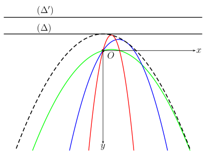
Figure 1: A few trajectories corresponding to various shooting angles in a constant gravitational field, and their envelope (dotted line).

2.2 Geometric solution

The parabolas (2) have in common a point $O$, and their directrix, $\Delta$, which is located at $y=-a/2$. The equation can, indeed, be read as

$$(y+a/2)^{2}=(x-x_{F})^{2}+(y-y_{F})^{2}~{},\quad x_{F}=-a\sin(2\alpha)/2,\ y_{F}=a\cos(2\alpha)/2~{},$$ (4)

revealing the focus $F$ located at $(x_{F},y_{F})$, i.e., on a circle, with centre at $O$, of radius $a/2$, at an angle $\beta=2\alpha-\pi/2$ with the horizontal.

The geometric construction follows, as shown in Fig. 2.

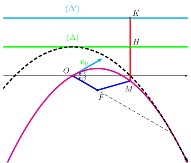
Figure 2: Geometrical construction of the envelope of the ballistic parabolas.

A current point $M$ of a trajectory fulfills $MF=MH$, with the notation of the figure. If $\Delta^{\prime}$ is parallel to the common directrix $\Delta$, at a distance $a/2$ further up, then the distance $MK$ to $\Delta^{\prime}$ and the distance $MO$ to the origin obey

$$MO\leq MF+FO=MH+HK=MK~{},$$ (5)

this demonstrating that the points within reach of the gun lie within a parabola of focus $O$ and directrix $\Delta^{\prime}$. The equality is satisfied when $M$, $F$ and $O$ are aligned. From $\beta=2\alpha-\pi/2$, a result pointed out by Macklin [5] is recovered, that the tangent to the envelope is perpendicular to the initial velocity of the trajectory that is touched. (If $M$ is on the envelope, $MO=MK$ and the tangent is the inner bisector of $\widehat{OMK}$.)

2.3 A family of circles

A more peaceful view at the safe domain is that of an ideal firework: projectiles of various angle $\alpha$ are fired all at once, with the same velocity [2]. At a given time $t$, they describe a circle (a sphere in space)

$$x^{2}+(y-ft^{2}/(2m))^{2}=(v_{0}t)^{2}~{},$$ (6)

with the centre at $\{0,ft^{2}/(2m)\}$, i.e., falling freely, and a growing radius $v_{0}t$. The problem of safety now consists of examining whether Eq. (6) has any solution in $t$ for given $x$ and $y$. This is a mere second-order equation, whose vanishing discriminant leads back to the parabola (3). Figure 3 show a few circles whose envelope is this parabola.

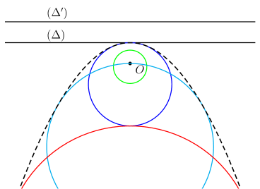
Figure 3: The safety parabola can be seen as surrounding the circles made at a given time $t$ by the projectiles shoot at once in all directions with the same velocity. For small $t$, the circle does not touch the safety parabola.

3 Coulomb or Kepler motion

3.1 Family of satellites

Let us consider an attractive Coulomb or Kepler potential $V=-K/r$, $K>0$, centered in $O$. If a particle of mass $m$ is fired from $A$ $(r_{0},0)$, with a velocity $\boldsymbol{v}_{0}$, whose angle with $OA$ is $\alpha$, then the trajectory obeys the equation [7]

$$u^{\prime\prime}+u={mK\over\mathcal{L}^{2}}~{},\quad u(0)={1\over r_{0}}~{},\quad u^{\prime}(0)=-{\cos\alpha\over r_{0}\sin\alpha}~{},$$ (7)

where $\mathcal{L}=mr_{0}v_{0}\sin\alpha$ is the orbital momentum, which is proportional to the constant areal velocity, and $u=1/r$, $u^{\prime}={\rm d}u/{\rm d}\theta$, etc. The solution is thus

$$u={K(1-\cos\theta)\over mr_{0}^{2}v_{0}^{2}\sin^{2}\alpha}+{\cos\theta\over r_{0}}-{\sin\theta\cos\alpha\over r_{0}\sin\alpha}~{},$$ (8)

A few trajectories are shown in Fig. 4, together with their envelope, which is an ellipse with foci, $O$, the centre of force, and $A$, the common starting point.

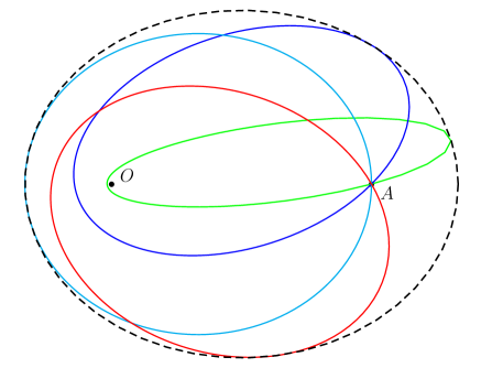
Figure 4: Trajectories of satellites launched from $A$ with the same velocity, but different initial direction. The envelope(dotted line) is an ellipse of foci $O$ and $A$.

The envelope is easily derived by elementary calculus. Equation (8), for a given point characterized by $u$ and $\theta$, should have acceptable solutions in $\alpha$. This is a mere second order equation in $\cot\alpha$, and the vanishing of its discriminant gives the border of the safe domain.

A geometric derivation of the envelope gives an answer even faster. All trajectories have same energy, and hence the same axis $2a$, since $E=-K/(2a)$ [7]. Hence the second focus, $F$ is on a circle of centre $A$, and radius $2a-r_{0}$. The initial velocity is one of the bisectors of $\widehat{OAF}$. For any point $M$ on the trajectory,

$$MO+MA\leq MO+MF+FA=4a-r_{0}~{},$$ (9)

which proves the property. One further sees that the envelope is touched when $M$, $F$ and $A$ are aligned. This is illustrated in Fig. 5.

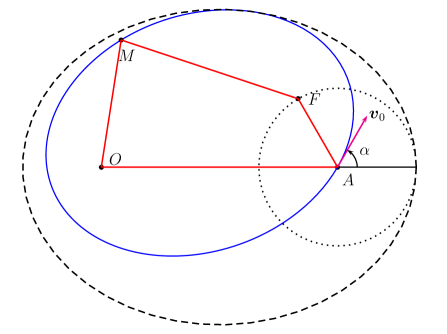
Figure 5: Geometric construction of the envelope of trajectories of satellites launched from $A$ with the the same velocity in various directions.

3.2 Rutherford scattering

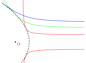
Figure 6: Trajectories in a repulsive Coulomb potential with same velocity but varying impact parameter.

As a variant, consider now the case of a repulsive interaction, $V=K/r$, $K>0$, as in Rutherford’s historical experiment. The simplest case is that of particles sent from very far away with the same velocity $\boldsymbol{v}_{0}$ but different values of the impact parameter $b$, this resulting in varying orbital momenta $\mathcal{L}$. Examples are shown in Fig. 6. We have a family of hyperbolas

$$u=-{a(1-\cos\theta)\over b^{2}}+{\sin\theta\over b}~{},$$ (10)

where $a=K/(mv_{0}^{2})$. This second-order equation in $b^{-1}$ has real solutions if

$$u\leq{1+\cos\theta\over 4a}~{},$$ (11)

corresponding to the outside of a parabola of focus $O$, also shown in Fig. 6.

The geometric interpretation is the following. All trajectories have the same energy $E=mv_{0}^{2}/2$, and hence the same axis $2a$ since $E=K/(2a)$, very much analogous to $E=-|K|/(2a)$ for ellipses in the case of attraction and negative energy. Each hyperbola has a focus $O$, and second focus $F$ on the line $\Delta$, perpendicular to the initial asymptote at distance $2a$ from $O$. The middle of $OF$ lies on this asymptote, whose position is determined by the impact parameter $b$. Let $\Delta^{\prime}$ be parallel to $\Delta$, at a further distance $2a$. If $M$ is on a trajectory, and is projected on $\Delta^{\prime}$ at $K$, then

$$MK-MO\leq MF+2a-MO=0~{},$$ (12)

with saturation when $M$, $F$ and $K$ are aligned. See Fig. 7.

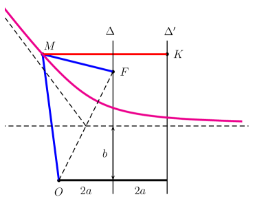
Figure 7: Geometric proof that the Rutherford trajectories with the same energy delimit a safe region.

3.3 Scattering from finite distance

A simple generalization consists of considering particles launched in the repulsive Coulomb field from a point $A$, at finite distance $r_{0}$ from the centre of force $O$. The kinetic energy, written as $mv_{0}^{2}/2=K/(2a)$, fixes the length scale $a$. The problem has been studied, e.g., by Samengo and Barrachina [6], who discussed glory- and rainbow-like effects. Some trajectories and their envelope and shown in Fig. 8. It can be seen, and proved that

• For $r_{0}>2a$, the envelope is a branch of hyperbola with $O$ as the inner focus. In the limit $r_{0}\to\infty$, we obtain the parabola of ordinary Rutherford scattering.

• For $r_{0}=2a$, the envelope is simply the mediatrix of $OA$.

• For $r_{0}<2a$, the envelope is a branch of hyperbola with $O$ as the external focus.

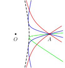
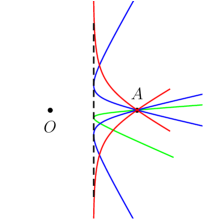
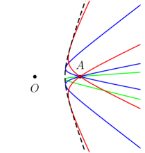
Figure 8: Rutherford scattering from $r_{0}=5a/2$ (left), $r_{0}=2a$ (centre) and $r_{0}=3a/2$ (right). The envelope is shown as a dotted line.

4 Harmonic potential

4.1 Firing in various directions

We now consider a particle of mass $m$ in a potential $kr^{2}/2$. Figure 9 shows a few trajectories from $A$, located at $(x_{0},0)$, with an initial velocity $\boldsymbol{v}_{0}$ of given modulus and varying angle.

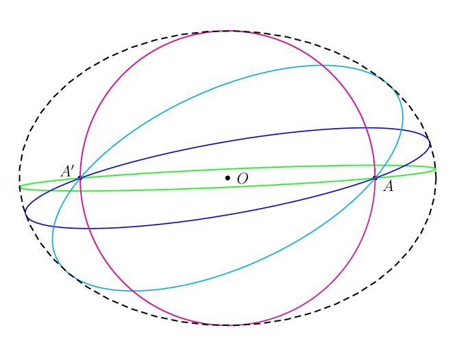
Figure 9: Trajectories in a harmonic potential with varying angle for the initial velocity.

This central-force problem is more easily solved directly in Cartesian coordinates, in contrast with most central forces problems, for which the use of polar coordinates is almost mandatory. One obtains

$$x(t)=x_{0}\cos(\omega t)+\ell_{0}\cos\alpha\sin(\omega t)~{},\quad y(t)=\ell_{0}\sin\alpha\sin(\omega t)~{},$$ (13)

where $\omega=\sqrt{k/m}$ and $\ell_{0}=v_{0}/\omega$, or, equivalently, the algebraic equation

$$\left({x-y\cot\alpha\over x_{0}}\right)^{2}+\left({y\over\ell_{0}\sin\alpha}\right)^{2}=1~{},$$ (14)

which can be read as a second-order equation in $\cot\alpha$. The condition to have real solutions for given $x$ and $y$ defines a domain limited by the ellipse

$${x^{2}\over x_{0}^{2}+\ell_{0}^{2}}+{y^{2}\over\ell_{0}^{2}}=1~{},$$ (15)

with centre $O$ and foci $A$, and its symmetric $A^{\prime}$. The points $A$ and $A^{\prime}$ belong to all trajectories. This envelope is also shown in Fig. 9.

4.2 Firing all projectiles simultaneously

The “fireball” view point leads to similar equations. If all projectiles are fired all at once, they describe, in a plane, at time $t$, the circle

$$(x-x_{0}\cos(\omega t))^{2}+y^{2}=\ell_{0}^{2}\sin^{2}(\omega t)~{},$$ (16)

whose radius $|\ell_{0}\sin(\omega t)|$ and centre position $x_{0}\cos(\omega t)$ oscillate. For given $x$ and $y$, this is, again, a second-order polynomial, now in $\cos(\omega t)$, and from its discriminant, the equation (15) of the envelope is recovered. Figure 10 shows the envelope surrounding the circles and touching some of those.

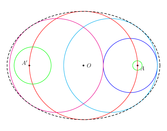
Figure 10: The projectiles, submitted to an harmonic potential centered at $O$, are all fired at $t=0$ with the same velocity, but in different directions. At any future time $t$, they describe a circle (a sphere in space) oscillating back and forth between $A$ and $A^{\prime}$ with a radius of varying length.

4.3 Geometric construction

The geometric construction of this envelope can be carried out as follows. All trajectories have again the same energy, $E=k(x_{0}^{2}+\ell_{0}^{2})/2$, since only the angle of the initial velocity is varied. This means that all ellipses have same quadratic sum $a^{2}+b^{2}$ of semi-major and semi-minor axes. There exists, indeed, a basis, where, after shifting time, the motion reads $X=a\cos(\omega t)$, $Y=b\sin(\omega t)$. If one recalculates the energy in this basis at $t=0$, one finds a potential term $ka^{2}/2$ and a kinetic term $m\omega^{2}b^{2}/2$, and hence $E=k(a^{2}+b^{2})/2$.

Now, if $M$ a running point of a trajectory $T$

$$MA+MA^{\prime}\leq\sup_{P\in T}(PA+PA^{\prime})=2\sqrt{x_{0}^{2}+\ell_{0}^{2}}~{},$$ (17)

corresponding, indeed, to an ellipse of foci $A$ and $A^{\prime}$.

A theorem is used here, that is not too well known, though it turns out (after several investigations of the author) that it is at the level of next-to-elementary geometry. It is described below.

4.4 A theorem on ellipses

Theorem: If $A\in T$ and $A^{\prime}\in T$ form a diameter of an ellipse $T$, and $M$ denotes a running point of $T$, the maximum of the sum of distances

$$\sup_{M\in T}(MA+MA^{\prime})~{},$$ (18)

is independent of $A$, with value $2\sqrt{a^{2}+b^{2}}$, where $a$ and $b$ denote the semi transverse and conjugate axes of $T$.

The proof can be found in Ref. [8, p. 350]. It is linked to a consequence of the Poncelet theorem formulated by Chasles.

Steps in understanding the above property include:

• The maximum is reached twice, for say, $M$ and $M^{\prime}$, $AMA^{\prime}M^{\prime}$ forming a parallelogram, as shown in Fig. 11.

• By first order variation, the tangent in $M$ is a bissectrix of $\widehat{AMA^{\prime}}$.

• The tangent in $M$ is perpendicular to the tangent in $A$. This provides the non-trivial result that if $M$ maximizes $MA+MA^{\prime}$, conversely, $A$ (or $A^{\prime}$) maximizes the sum of distances to $M$ and $M^{\prime}$.

• The tangents in $A$, $M$, $A^{\prime}$, and $M^{\prime}$ forming a rectangle, the Monge theorem [8, p. 332] applies, stating that the orthoptic curve of the ellipse (set of points from which the ellipse is seen at 90^∘), is a circle of radius $\sqrt{a^{2}+b^{2}}$, see Fig. 11.

• The sides of the parallelogram $AMA^{\prime}M^{\prime}$ are tangent to an ellipse $T^{\prime}$ with same foci as $T$, but flattened, with semi-axes

  $$a^{\prime}={a^{2}\over\sqrt{a^{2}+b^{2}}}~{},\quad b^{\prime}={a^{2}\over\sqrt{a^{2}+b^{2}}}~{}.$$ (19)

Figure 11: An ellipse of semi-axes $a$ and $b$, a diameter $AA^{\prime}$ and the points $M$ and $M^{\prime}$ such as $MA+MA^{\prime}$ is maximal. The result is independent of $A$. The tangents in $A$ and $M$ are orthogonal, and thus intersect on the orthoptic curve of the ellipse, which is a circle. The sides of the parallelogram are tangent to a homofocal ellipse of semi-axes $a^{2}/\sqrt{a^{2}+b^{2}}$ and $b^{2}/\sqrt{a^{2}+b^{2}}$.

Note that if one tries to demonstrate this theorem by straightforward calculus, one generally writes down cumbersome equations. One of the simplest – if not the simplest – methods, would consist of starting from the trajectories (13), identifying there the most general set of ellipses of given $a^{2}+b^{2}$, and calculating the envelope (15), which is easily identified as an ellipse of foci $A$ and $A^{\prime}$ and major axis $2\sqrt{a^{2}+b^{2}}$. It thus follows that on each trajectory, $MA+MA^{\prime}\leq 2\sqrt{a^{2}+b^{2}}$, with saturation when the trajectory touches its envelope.

5 Conclusions

Conic sections are encountered in classical optics, where they provide a design for ideal mirrors with perfect refocusing properties of light rays emitted by a suitably-located point-source.

Trajectories in elementary mechanics simple potentials such as a linear, Coulomb or quadratic potential, also follow conic sections. When the angle of the initial velocity is varied, one gets a family of trajectories with the same total energy. Their envelope sets the limits of the safe domain. This envelope can be deduced by recollecting astute though somewhat old-fashioned methods of geometry courses.

If the potential becomes more complicated or if one uses relativistic kinematics, the envelope has to be derived by calculus, but the techniques can be probed first on these cases where a purely geometric solution is available.

Acknowledgements

Useful information from X. Artru, J.-P. Bourguignon, A. Connes and M. Berger, and comments by A.J. Cole are gratefully acknowledged.

References

- [1] See, for instance, A. González-Villanueva, E. Guillaumín-España, R.P. Martínez-y-Romero, H.N. Núñez-Yépez and A. L. Salas-Brito, Eur. J. Phys. 19, 431 (1998); S.K. Bose, Am. J. Phys. 53, 175 (1985); D. Derbes, Am. J. Phys. 69, 481 (2001); Th.A. Apostolatos, Am. J. Phys. 71 261 (2003); D.M. Williams, Am. J. Phys. 71, 1198 (2003); and references therein.
- [2] D. Donnelly, Am. J. Phys. 60, 1149 (1992).
- [3] A.P. French, Am. J. Phys. 61, 805 (1993).
- [4] R.E. Warner and L.A. Huttar, Am. J. Phys. 59, 755 (1991).
- [5] Ph.A. Macklin, Am. J. Phys. 55, 947 (1987).
- [6] I. Samengo and R.O. Barrachina, Eur. J. Phys. 15, 300 (1994).
- [7] See, for instance, H. Goldstein, Ch. Poole and J. Safko, Classical Mechanics, 3rd ed. (Addison-Wesley, New-York, 2002).
- [8] M. Berger, Géométrie, Tome 2 (Nathan, Paris, 1990).