On dynamical tunneling and classical resonances

Abstract

This letter establishes a firm relationship between classical nonlinear resonances and the phenomenon of dynamical tunneling. It is shown that the classical phase space with its hierarchy of resonance islands completely characterizes dynamical tunneling. In particular, it is not important to invoke criteria such as the size of the islands and presence or absence of avoided crossings for a consistent description of dynamical tunneling in near-integrable systems.

Dynamical tunneling as a concept emerged more than two decades ago in the field of chemical physics where it results in the transport of vibrational quanta between degenerate modes - a process that would be classically forbidden. The importance of dynamical tunneling in the molecular context can be hardly overstated since this phenomenon provides a route to energy flow through the molecule in the absence of direct classically resonant mechanisms. Early pioneering worklawch ; davhel ; husihy ; stumar ; orti mainly by the chemical physics community provided both semiclassicallawch ; davhel and purely quantum perspectiveshusihy ; stumar on dynamical tunneling. Semiclassically the phase space is the natural setting whereas the quantum approach invokes high order perturbation theory involving a chain of off-resonant virtual states (vibrational superexchangestumar ). Although seemingly different, there are hintsstumar ; self towards a connection between the two perspectives and this paper attempts to provide further clues.

The initial suggestiondavhel regarding the importance of phase space structures to dynamical tunneling has been intensely studied and established by the nonlinear dynamics community over the last decadeozo ; cat ; cats ; rat1 ; rat2 ; frido . Dynamical tunneling is found not only to be influenced by chaoscat ; cats ; frido but also by various nonlinear resonancesrat1 ; rat2 ; frido ; self with some recent experimental supportexpt . In the molecular context Heller recentlyejhsar made a number of interesting observations and conjectures on the possible implications of dynamical tunneling on high resolution molecular spectralehm . The most important amongst these is the claim that a nominal 10^-1-10^-2 cm^-1 broadening of spectroscopically prepared zeroth order states is due to dynamical tunneling between remote regions of phase space facilitated by distant resonances. Arguments were provided for identifying the specific resonances and subsequent calculation of the splittings. The purpose of this letter is to confirm the above claim via a detailed analysis of a relatively simple, albeit realistic, model spectroscopic Hamiltonian. The analysis also indicates that the correspondence between classical resonances and avoided crossings, while interesting, is not needed for an understanding of dynamical tunneling.

We use a model spectroscopic Hamiltonianksjcp

$$\hat{H}=\hat{H}_{0}+g\hat{V}^{(12)}_{1:1}+\gamma\hat{V}^{(12)}_{2:2}+\beta(\hat{V}^{(1b)}_{2:1}+\hat{V}^{(2b)}_{2:1})$$ (1)

with

$$\hat{H}_{0} = \omega_{s}(n_{1}+n_{2})+\omega_{b}n_{b}+x_{s}(n^{2}_{1}+n^{2}_{2})$$ (2)

$$+ x_{b}n^{2}_{b}+x_{sb}n_{b}(n_{1}+n_{2})+x_{ss}n_{1}n_{2}$$

The values of these parameters, in cm^-1, $\omega_{s}=3885.57,\omega_{b}=1651.72,x_{s}=-81.99,x_{b}=-18.91,x_{ss}=-12.17$, and $x_{sb}=-19.12$ are representative of the H₂O moleculebag . The three anharmonic modes are labeled as stretches $(1,2)$ and a bend $(b)$ and $\hat{H}$ is symmetric under $1\leftrightarrow 2$. The $j^{th}$ mode occupancy is $n_{j}=a^{\dagger}_{j}a_{j}$ with $(a^{\dagger}_{j},a_{j})$ denoting the usual harmonic oscillator creation and destruction operators for mode $j$. The various perturbations $\hat{V}^{(ij)}_{p:q}=(a^{\dagger}_{i})^{q}(a_{j})^{p}+h.c.$ connect zeroth-order states $|{\bf n}\rangle$, $|{\bf n}^{\prime}\rangle$ with $|n_{i}^{\prime}-n_{i}|=q$ and $|n_{j}^{\prime}-n_{j}|=p$. The classical limitksjcp of the above Hamiltonian is a nonlinear multiresonant Hamiltonian $H({\bf I},{\bm{\theta}})$ with $(I_{j},\theta_{j})$ corresponding to the action-angle variables associated with the mode $j$. In particular the classical limit of $\hat{V}^{(ij)}_{p:q}$ is of the form $2\sqrt{I_{i}^{q}I_{j}^{p}}\cos(q\theta_{i}-p\theta_{j})$. $\hat{H}$ can be obtained by a fit to the high resolution experimental spectra or from a perturbative analysis of a high quality ab initio potential energy surface. In either case such effective Hamiltonians provide a very natural and convenient representation to understand the spectral patterns of molecular systemshrs . Note that despite the three coupled modes, $\hat{H}$ is effectively two dimensional due to the existence of the conserved quantity $P=(n_{1}+n_{2})+n_{b}/2$ called as the polyad number. The classical Hamiltonian is integrable if $\beta=0$ and for our choice of parameters it is near-integrable if $\beta\neq 0$. Throughout this study we fix $P=8$ and $\beta=26.57$ cm^-1 and denote, due to conserved $P$, the zeroth-order states by $|n_{1},n_{2}\rangle$.

Figure 1: State or zeroth-order number space with the location and width of the 2:1 resonance zones. An example superexchange path (dashed) between the degenerate states $|2,0\rangle$ and $|0,2\rangle$ is indicated. The inset shows the survival probability for $|2,0\rangle$ and $|0,2\rangle$ (symbols) versus time.

To begin with consider the case wherein only the 2:1 resonances are present i.e., $g=\gamma=0$. In order to emphasize and illustrate the concept we choose the zeroth-order degenerate states $|2,0\rangle$ and $|0,2\rangle$ without loss of generality. Since $\langle 2,0|\hat{V}^{(1b)}_{2:1}|0,2\rangle=0=\langle 2,0|\hat{V}^{(2b)}_{2:1}|0,2\rangle$ the state $|2,0\rangle$ is uncoupled from the symmetric counterpart $|0,2\rangle$. However, dynamical tunneling can mix these states and indeed from Fig. 1 one observes a coherent transfer of population with a period of about $0.15$ ns corresponding to to a splitting $\Delta_{2}\approx 0.22$ cm^-1. The nontrivial nature of this process is amplified when one considers the fact that at the energy corresponding to $|2,0\rangle$ the primary 2:1 resonances are absent in the classical phase space. As shown in Fig. 1 the two states are far away in state space from the 2:1 primary resonance zones. One possible explanation of the tunneling arises from the perspective of high order perturbation theory or vibrational superexchangehusihy ; stumar . In this approach the states coupled locally by the 2:1 perturbations are considered and one constructs perturbative chains which connect the two states $|2,0\rangle$ and $|0,2\rangle$. An example of such a chain is $|2,0\rangle\rightarrow|1,0\rangle\rightarrow|1,1\rangle\rightarrow|0,1\rangle\rightarrow|0,2\rangle$. The contribution to the splitting from the chain is given by perturbation theory to be

$$\beta^{4}\frac{\langle 20|\hat{V}^{(1b)}|10\rangle\langle 10|\hat{V}^{(2b)}|11\rangle\langle 11|\hat{V}^{(1b)}|01\rangle\langle 01|\hat{V}^{(2b)}|02\rangle}{(\Delta E^{0}_{1,0,14})^{2}(\Delta E^{0}_{1,1,12})}$$ (3)

with $\Delta E^{0}_{n_{1},n_{2},n_{b}}\equiv E^{0}_{2,0,12}-E^{0}_{n_{1},n_{2},n_{b}}$. In principle there are an infinite number of chains that connect the two degenerate states. In practice, due to the energy denominators and near-integrability, it is sufficient to consider the minimal length chainsself . In our case there are six minimal chains and summing the contributions from each one of them one obtains a splitting of about $0.23$ cm^-1. This compares well with the exact splitting but it is important to note that all six perturbative terms have to be considered for this agreement. Note that although formally the superexchange approach invokes the resonant terms the connection to the classical phase space is lost. If indeed dynamical tunneling is properly understood in the phase space then surely there must be a phase space analog of the superexchange approach. The rest of the paper is dedicated to uncovering precisely such a phase space picture.

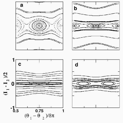
Figure 2: Surface of section at $E=E^{0}_{2,0,12}$ and $\beta=26.57$ cm^-1 for varying primary 1:1 strength in cm^-1. (a) $g=0$, (b) $g=-2.7$, (c) $g=-2.95\approx g_{0}$, and (d) $g=-3.4$. Note that for $g<g_{0}$ the island corresponds to the induced 1:1 whereas for $g>g_{0}$ the island correspond to the primary 1:1. Also note that a Husimi representation of the states $|2,0\rangle$ and $|0,2\rangle$ would be localized about $(I_{1}-I_{2})/2=\pm 1$ respectively.

As mentioned the primary 2:1 resonances do not appear in the phase space at $E=E^{0}_{2,0,12}$ and hence a direct involvement is ruled out. Nevertheless a weak overlap between the 2:1s can result in an induced 1:1 resonance which can then mediate dynamical tunneling between the states. In Fig. 2a we show the surface of section at $E=E^{0}_{2,0,12}$ and one indeed observes a resonance island between the two states. In order to confirm the nature of this resonance zone we use standard methods of nonlinear dynamicslicht to extract the necessary information. In essence one starts with the classical Hamiltonian involving only the 2:1 perturbations in the formksjcp

$$H({\bf J},{\bm{\psi}};N) = H_{0}({\bf J};N)+\epsilon\beta_{c}(N-2J_{1}-2J_{2})$$

$$\times [\sqrt{J_{1}}\cos\psi_{1}+\sqrt{J_{2}}\cos\psi_{2}]$$

with $\beta_{c}=\beta/\sqrt{2}$ and $N$ being the classical analog of the polyad number. A formal parameter $\epsilon$ has been introduced with the aim of perturbatively removing the 2:1 resonances, characterized by $\psi_{1,2}$, to $O(\epsilon)$. This can be done by invoking the generating function $F=\bar{J}_{1}\psi_{1}+\bar{J}_{2}\psi_{2}+\epsilon[g_{1}\sin\psi_{1}+g_{2}\sin\psi_{2}]$ where the functions $g_{1,2}=g_{1,2}(\bar{J}_{1},\bar{J}_{2})$ are determined by the condition of the removal of the primary 2:1s to $O(\epsilon)$. The angles conjugate to ${\bar{\bf J}}$ are denoted by ${\bar{\bm{\psi}}}$. The procedure is algebraically tedious and we skip the details to provide the important results. The choice of the functions $g_{1,2}$ turns out to be:

$$g_{1,2}(\bar{J}_{1},\bar{J}_{2})=-\beta_{c}\frac{(N-2\bar{J}_{1}-2\bar{J}_{2})\sqrt{\bar{J}_{1,2}}}{\Omega_{s}+2\alpha_{ss}\bar{J}_{1,2}+\alpha_{12}\bar{J}_{2,1}}$$ (5)

where $\Omega_{s}=\omega_{s}-2\omega_{b}+(x_{sb}-4x_{b})N,\alpha_{ss}=x_{s}+4x_{b}-2x_{sb}$ and $\alpha_{12}=8x_{b}-4x_{sb}+x_{ss}$. Using the above result it is possible to show that an induced 1:1 resonance appears at $O(\epsilon^{2})$ with a coefficient

$$g_{ind}=\frac{\beta_{c}^{2}}{2}(N-2\bar{J}_{1}-2\bar{J}_{2})f(\bar{J}_{1},\bar{J}_{2};N)\sqrt{\bar{J}_{1}\bar{J}_{2}}$$ (6)

with $f(\bar{J}_{1},\bar{J}_{2};N)$ being a complicated function of the actions. At this stage the transformed Hamiltonian to $O(\epsilon^{2})$ still depends on both the angles $\bar{\psi}_{1}$ and $\bar{\psi}_{2}$ and hence non-integrable. In order to isolate the induced 1:1 resonance we perform a canonical transformation to the variables $({\bf K},{\bm{\phi}})$ using the generating function $G=(\bar{\psi}_{1}-\bar{\psi}_{2})K_{1}/2+(\bar{\psi}_{1}+\bar{\psi}_{2})K_{2}/2$ and average the resulting Hamiltonian over the fast angle $\phi_{2}$. The resonance center, $K_{1}^{r}=0$, approximation is invoked resulting in a pendulum Hamiltonian describing the induced 1:1 resonance island structure seen in the surface of section shown in Fig. 2a. Within the averaged approximation the action $K_{2}=\bar{J}_{1}+\bar{J}_{2}$ is a constant of the motion and can be identified as the 1:1 polyad associated with the secondary resonance. The resulting integrable Hamiltonian is given by

$$\bar{H}(K_{1},\phi_{1};K_{2},N)=\frac{1}{2M_{11}}K_{1}^{2}+2g_{ind}(K_{2},N)\cos 2\phi_{1}$$ (7)

where

$$M_{11} = 2(\alpha_{12}-2\alpha_{ss})^{-1}$$ (8a)

$$g_{ind}(K_{2},N) = \frac{\beta_{c}^{2}}{2}\bar{f}(K_{2},N)(N-2K_{2})K_{2}$$ (8b)

with

$$\bar{f}(K_{2},N)=\frac{4(\Omega_{s}+\alpha_{ss}K_{2})+\alpha_{12}N}{[2(\Omega_{s}+\alpha_{ss}K_{2})+\alpha_{12}K_{2}]^{2}}$$ (8c)

In terms of the zeroth-order quantum numbers $K_{1}=n_{1}-n_{2}$ and $K_{2}=n_{1}+n_{2}+1\equiv m+1$.

One can now use the above pendulum Hamiltonian to calculate the resulting dynamical tunnel splitting of the degenerate modes $|n_{1}=r,n_{2}=0,n_{b}=2(P-r)\rangle$ and $|n_{1}=0,n_{2}=r,n_{b}=2(P-r)\rangle$ viastumar

$$\frac{\Delta^{sc}_{r}}{2}=g_{ind}\prod_{m=-(r-2)}^{(r-2)}\frac{g_{ind}}{E_{R}^{0}(r)-E_{R}^{0}(m)}$$ (9)

where $E_{R}^{0}(k)=k^{2}/2M_{11}$ is the zeroth-order energy. For our example with $r=2,m=2$ using the parameters of the Hamiltonian we find $M_{11}\approx 1.32\times 10^{-2}$ and $g_{ind}\approx 4.43$ cm^-1. The resulting splitting $\Delta_{2}^{sc}\approx 0.26$ cm^-1 agrees very well with the exact splitting. This proves that the induced 1:1 resonance arising from the interaction of the two primary 2:1 resonances is mediating dynamical tunneling between the degenerate states. At this juncture it is important to note that the induced resonance strength is quite small and the two states are not involved in any avoided crossing. Moreover, from a superexchange perspective it is illuminating to note that the splitting can be calculated trivially by recognizing the secondary phase space structure (a viewpoint emphasized in Ref. rat2, as well). In comparison the original superexchange calculation, without any reference to the phase space, required taking into account $6$ terms with varying signscomment . This observation emphasizes the superior nature of a phase space viewpoint on dynamical tunneling.

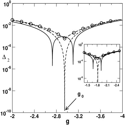
Figure 3: The variation of the dynamical splitting $\Delta_{2}$ with the primary 1:1 resonance strength $g$ is shown (solid line). The WKB estimate is shown as dashed line. WKB estimate with a small 2:2 resonance added is also shown (circles). The inset shows a similar calculation with a different set of parameters representing the D₂O moleculebag . In this case $\beta=15.78$ and, $g_{ind}\approx 2.73$ cm^-1.

As a further demonstration of the role of nonlinear resonances in dynamical tunneling we consider the Hamiltonian in eq. 1 with $g\neq 0$ with $\gamma=0$. In particular the sign of the primary 1:1 perturbation strength $g$ is taken to be the opposite of the induced 1:1 strength $g_{ind}$. If the induced resonance is playing a role then from our analysis we expect that the primary and induced resonances will cancel each other around $g=g_{0}\approx-2g_{ind}/(m+1)$ resulting in small splittings in this region. In Fig. 3 the exact splittings are shown as a function of $g$ with the WKB resultshusihy ; stumar for comparison. This confirms our expectations to a certain degree in that the splittings are undergoing dramatic changes in the vicinity of $g_{0}$. A crucial observation is that the exact splitting is orders of magnitude larger than the simple WKB estimate and become small slightly away from $g_{0}$. On the other hand the classical phase space in Fig. 2 indicates the predicted disappearance of the 1:1 islands. From our arguments this far it would be natural to associate one or more high order nonlinear resonances with the residual tunneling around $g_{0}$ since the simple semiclassical estimate for $g_{0}$ was based on the $O(\epsilon^{2})$ induced 1:1 resonance cancelling the primary 1:1 resonance. In reality there are the harmonics of the 1:1 resonance that appear at higher orders in $\epsilon$. It is expected that the strengths of such higher harmonics like 2:2, 3:3, etc. would be extremely small. Nevertheless around $g=g_{0}$ the most dominant resonance involved in dynamical tunneling would be the 2:2. The strength of this tiny but dominant 2:2 resonance can be estimated roughly by adding a 2:2 perturbation ($\gamma$) to eq. 1 with $\beta=26.57$ cm^-1, $g=g_{0}$ and noting the value of $\gamma$ for which the exact and WKB results come close. A much more rigorous estimate, which is a difficult excersise in classical perturbation theory, can be made by going to higher orders, atleast $O(\epsilon^{3})$, in $\epsilon$. We now estimate the splitting with a WKB calculation including the 2:2 resonance with strength $\gamma\approx 2.32355\times 10^{-4}$ cm^-1. It is clear from Fig. 3 that the exact splitting and the modified WKB estimate based on the higher order 2:2 agree fairly well. It is also satisfying to see that the modified WKB calculation hardly effects the splittings far away from $g=g_{0}$. As an independent check in Fig. 3(inset) we show the same calculation for a different set of $\hat{H}_{0}$ parameters representative of the D₂O moleculebag and the results are similar. This supports the argument that in the vicinity of $g_{0}$, where the 1:1 resonance is absent, the extremely small 2:2 resonance is mediating the dynamical tunneling between the states $|2,0\rangle$ and $|0,2\rangle$. Two remarks are in order at this stage. First the two states do not undergo any avoided crossing as a function of the parameter $g$. This can also be indirectly inferred from the fact that a superexchange calculation of the splittings essentially reproduces the exact result and thus include the importance of higher order resonances near $g=g_{0}$. A more detailed analysis of the perturbative chains from the semiclassical viewpoint would be interesting. Second the modified WKB calculation is in good agreement with the exact splittings only in the vicinity of $g_{0}$ by necessity. There are contributions from even higher order resonances which are absent from our simplified analysis and a subtle interplay of all the nonlinear resonances give rise to the exact result.

To summarize, in this work using a model spectroscopic Hamiltonian we have demonstrated the intimate connection between dynamical tunneling and the resonance structure of the classical phase space. Thus dynamical tunneling connects two degenerate states as long as there is a nonlinear resonance juxtaposed between them as viewed in the phase space. The order and width of the resonance are immaterial. This supports an earlier claim regarding the possibility of dynamical tunneling as a source of narrow spectral clusters associated with spectroscopically prepared, localized, zero-order states. However the notion that such resonances are the cause of avoided crossings does not seem to hold. Consequently it is also not necessary that only a specific classical resonance be the agent of dynamical tunneling. Primary, induced and even higher harmonics of the resonances can mediate dynamical tunneling and the consequences for energy flow and control from this standpoint seem crucial and needs further study. It is interesting to note that in multidimensional near-integrable systems nonlinear resonances would be involved in two long time phenomena - dynamical tunneling and Arnol’d diffusionlicht . The competition between them and their spectral consequences are worth investigating from a fundamental standpointcompet .

It is a pleasure to thank Peter Schlagheck for critical and illuminating discussions. I am grateful to Prof. Klaus Richter for the hospitality and support at the Universität Regensburg where this work was done.

References

- (1) R. T. Lawton and M. S. Child, Mol. Phys. 37, 1799 (1979).
- (2) M. J. Davis and E. J. Heller, J. Chem. Phys. 75, 246 (1981).
- (3) J. S. Hutchinson, E. L. Sibert III, and J. T. Hynes, J. Chem. Phys. 81, 1314 (1984).
- (4) A. A. Stuchebrukhov and R. A. Marcus, J. Chem. Phys.98, 8443 (1993).
- (5) S. Keshavamurthy, J. Chem. Phys. 119, 161 (2003).
- (6) M. E. Kellman, J. Chem. Phys. 76, 4528 (1982); W. G. Harter and C. W. Patterson, J. Chem. Phys. 80, 4241 (1984); J. Ortigoso, Phys. Rev. A 54, R2521 (1996).
- (7) A. M. Ozorio de Almeida, J. Phys. Chem. 88, 6139 (1984).
- (8) O. Bohigas, S. Tomsovic, and D. Ullmo, Phys. Rep. 223, 43 (1993).
- (9) Tunneling in Complex Systems, edited by S. Tomsovic (World Scientific, Singapore, 1998) and references therein; W. A. Lin and L. E. Ballentine, Phys. Rev. Lett. 65, 2927 (1990); R. Utermann, T. Dittrich, and P. Hänggi, Phys. Rev. E 49, 273 (1994); A. Shudo and K. S. Ikeda, Phys. Rev. Lett. 76, 4151 (1996); S. C. Creagh and N. D. Whelan, Phys. Rev. Lett. 77, 4975 (1996).
- (10) R. Roncaglia, L. Bonci, F. M. Izrailev, B. J. West, and P. Grigolini, Phys. Rev. Lett. 73, 802 (1994); L. Bonci, A. Farusi, P. Grigolini, and R. Roncaglia, Phys. Rev. E 58, 5689 (1998).
- (11) O. Brodier, P. Schlagheck, and D. Ullmo, Phys. Rev. Lett. 87, 064101 (2001); O. Brodier, P. Schlagheck, and D. Ullmo, Ann. Phys. 300, 88 (2002); C. Eltschka and P. Schlagheck, nlin.CD/0409016 (2004).
- (12) E. Doron and S. D. Frischat, Phys. Rev. Lett. 75, 3661 (1995); S. D. Frischat and E. Doron, Phys. Rev. E 57, 1421 (1998).
- (13) J. Zakrzewski, D. Delande, and A. Buchleitner, Phys. Rev. E 57, 1458 (1998); J. U. Nöckel and A. D. Stone, Nature 385, 45 (1997); W. K. Hensinger, H. Häffner, A. Browaeys, N. R. Heckenberg, K. Helmerson, C. Mckenzie, G. J. Milburn, W. D. Phillips, S. L. Roston, H. Rubinsztein-Dunlop, and B. Upcroft, Nature 412, 52 (2001); D. A. Steck, W. H. Oskay, and M. G. Raizen, Science 293, 274 (2001); A. P. S. de Moura, Y-Cheng Lai, R. Akis, J. P. Bird, and D. K. Ferry, Phys. Rev. Lett. 88, 236804 (2002).
- (14) E. J. Heller, J. Phys. Chem. 99, 2625 (1995).
- (15) E. R. Th. Kerstel, K. K. Lehmann, T. F. Mentel, B. H. Pate, and G. Scoles, J. Phys. Chem. 95, 8282 (1991); T. K. Minton, H. L. Kim, S. A. Reid, and J. D. McDonald, J. Phys. Chem. 89, 6550 (1988); A. McIlroy and D. J. Nesbitt, J. Chem. Phys. 91, 104 (1989); See M. Gruebele, J. Phys.: Condens. Matter 16, R1057 (2004) for more possible experimental fingerprints of dynamical tunneling in high resolution molecular spectra.
- (16) The Hamiltonian used here is adapted from the one analyzed in S. Keshavamurthy and G. S. Ezra, J. Chem. Phys. 107, 156 (1997); S. Keshavamurthy and G. S. Ezra, Chem. Phys. Lett. , (1995).
- (17) J. E. Baggot, Mol. Phys. 65, 739 (1988).
- (18) M. Gruebele, Adv. Chem. Phys. 114, 193 (2000); G. S. Ezra, Adv. Class. Traj. Meth. 3, 35 (1998).
- (19) See for example, A. J. Lichtenberg and M. A. Lieberman, Regular and Chaotic Dynamics, Springer-Verlag, New York, 1992.
- (20) This observation is quite dramatic whe one considers the dynamical tunneling between and . In this case the superexchange approach involves terms with varying signs and gives cm-1 and the phase space approach again involves only one term yielding cm-1. For comparison the exact splitting cm-1.
- (21) Some work has been done along this line. See E. Tannenbaum, Ph.D. thesis, chapter 3, Harvard University, 2002.