Criteria for the experimental observation of multi-dimensional optical solitons in saturable media

Abstract

Criteria for experimental observation of multi-dimensional optical solitons in media with saturable refractive nonlinearities are developed. The criteria are applied to actual material parameters (characterizing the cubic self-focusing and quintic self-defocusing nonlinearities, two-photon loss, and optical-damage threshold) for various glasses. This way, we identify operation windows for soliton formation in these glasses. It is found that two-photon absorption sets stringent limits on the windows. We conclude that, while a well-defined window of parameters exists for two-dimensional solitons (spatial or spatiotemporal), for their three-dimensional spatiotemporal counterparts such a window does not exist, due to the nonlinear loss in glasses.

I Introduction

Solitons are localized wave packets and/or beams that result from the balance of the linear and nonlinear responses of a physical system. Depending on the physical properties of the underlying system, solitons take different forms. They can be hydrodynamic wave packets, such as solitary waves in the ocean solocean and atmosphere solatom . They can also be spin-wave packets, such as magnetic solitons spinsol1 ; spinsol2 . Bose-Einstein condensates provide a medium to produce matter-wave solitons becsol . Other examples of soliton dynamics can be found in a wide variety of fields, including astrophysics, plasma physics, nuclear physics, and even metabolic biology astro1 ; astro2 ; nucle1 ; bio1 , among others. Very accurate experiments have been performed with topological solitons (fluxons) in long Josephson junctions, including a recent direct observation of their macroscopic quantum properties Ustinov .

Solitons in optics, which are known in their temporal, spatial, and spatiotemporal varieties (the latter ones being frequently called “light bullets”), constitute, perhaps, the most versatile and well-studied (both theoretically and experimentally) class of solitons in physics. In particular, temporal solitons in optical fibers agrawal have recently made a commercial debut in high-speed telecommunications links agrawal ; Australia . It has been pointed out that multi-dimensional (multi-D) spatiotemporal optical solitons can be used in the design of high-speed all-optical logic gates and, eventually, in all-optical computation and communications systems soliton_gate .

The balance of linear and nonlinear dynamical features is only the first step in the soliton formation. Securing the stability of this balance is the second, equally important step. A well-known difficulty is that the most common optical nonlinearity – the Kerr effect in dielectrics – gives rise to soliton solutions which are unstable in more than one dimension against the wave collapse, as discussed (in particular) in original papers jetpcollapse ; soliton_collapse4 and in the review Luc . Several mechanisms that can suppress the collapse have been investigated. These include saturation of the Kerr nonlinearity satkerr , higher-order dispersion or diffraction (also referred to as ”non-paraxiality”) non_parax , multiphoton ionization multi-photon , and stimulated Raman scattering (SRS) srs1 ; srs2 . In particular, importance of the multi-photon absorption and SRS for the spatiotemporal self-focusing of light in the Kerr medium was inferred from experimental data in Ref. Shimshon . However, these mechanisms eventually reduce the intensity and cause the pulse to expand in time and space, precluding the achievement of multi-dimensional solitons frank .

Different versions of the saturable nonlinearity (which implies saturation of the cubic nonlinear susceptibility, $\chi^{(3)}$, in high-intensity fields) have been studied theoretically in detail. It was shown that both rational yc ; enns_1 ; edmundson_1 ; edmundson_2 ; blair and cubic-quintic (CQ) quiroga ; Anton ; boris variants of the saturation readily support stable two-dimensional (2D) and three-dimensional (3D) solitons. A difference between them is that the former cannot stabilize “spinning” solitons with an intrinsic vorticity, but the CQ nonlinearity makes it possible, in the 2D Spain ; Lucian ; BobPego and even 3D spinning-bullet cases.

The first observation of a self-trapped beam in a Kerr medium was reported by Bjorkholm and Ashkin in 1974 bj . The experiment was done in sodium vapor around the $D_{2}$ transition line, and self-focusing arose from strong saturation of the transition (i.e. saturation of the linear susceptibility, $\chi^{(1)}$). Studies of 2D solitons have made rapid progress since the mid-1990’s in the study of two new nonlinearities featuring saturation. Segev et al. predicted that the photorefractive (PR) effect in electro-optic materials could be exploited to create an effective saturable nonlinear index of refraction that would support solitons segevprl . PR solitons were observed experimentally soon afterward duree . In parallel to this, there was a resurgence of interest in the so-called cascading nonlinearity, which is produced by the interaction of two or three waves in media with quadratic ($\chi^{(2)}$) nonlinear susceptibility. Both 1D and multi-D solitons in the quadratic media had been studied theoretically in numerous works (see reviews Jena and buryak ). Stationary 2D spatial solitons (in the form of self-supporting cylindrical beams) were first generated in quadratic media by Torruellas et al. torru . Later, Di Trapani et al. observed temporal $\chi^{(2)}$ solitons tquadratic , and, finally, spatiotemporal solitons were produced by Liu et al. quadratic_sts ; quadratic_sts2 . Under appropriate conditions, both the PR and cascading nonlinearities may be modeled as saturable generalizations of the Kerr nonlinearity (despite the fact that the PR media are, strictly speaking, non-instantaneous, nonlocal, and anisotropic). However, to date, multi-D solitons in true saturable Kerr media have not been observed.

In this work, we examine the possibility of stabilizing solitons (arresting the collapse) in saturable Kerr media satkerr , from the perspective of experimental implementation. Existing theories provide for parameter regions where formation of stable solitons is possible, but neglect linear and nonlinear losses, as well as other limitations, such as optical damage in high-intensity fields footnote . First, we propose a criterion for acceptable losses, and determine the consequences of the loss for the observation of soliton-like beams and/or pulses.

Then, as benchmark saturable Kerr media, we consider nonlinear glasses. Direct experimental measurements of the higher-order nonlinearities and nonlinear (two-photon) loss in a series of glasses allow us to link the theoretical predictions to experimentally relevant values of the parameters. As a result, we produce “maps” of the experimental-parameter space where 2D and 3D solitons can be produced. To our knowledge, this is the first systematic analysis of the effects of nonlinear absorption on soliton formation in saturable Kerr media. We conclude that it should be possible, although challenging, to experimentally produce 2D spatial and 2D spatiotemporal solitons in homogeneous saturable media. Spatiotemporal solitons require anomalous group-velocity dispersion (GVD). Under conditions relevant to saturation of the Kerr nonlinearity, material dispersion is likely to be normal. In that case, anomalous GVD might be obtained by pulse-tilting e.g. On the other hand, the prospects for stabilizing 3D solitons seem poor, even ignoring the need for anomalous GVD. This conclusion suggests that qualitatively different nonlinearities, such as $\chi^{(2)}$, may be more relevant to making light bullets.

We focus on Gaussian beam profiles, which are prototypical localized solutions. Very recent work has shown that nonlinear loss can induce a transition from Gaussian to conical waves, which can be stationary and localized filinochannel ; arxiv . The conical waves are very interesting, but represent a different regime of wave propagation from that considered here.

The rest of the paper is organized as follows. The theoretical analysis of the necessary conditions for the formation of the 2D and 3D solitons is presented in Section 2. Results of experimental measurements of the nonlinear parameters (cubic and quintic susceptibilities, and two-photon loss) in a range of glasses are reported in Section 3. Final results, in the form of windows in the space of physical parameters where the solitons may be generated in the experiment, are displayed in Section 4, and the paper is concluded by Section 5.

II Theoretical analysis of necessary conditions for the existence of two- and three-dimensional solitons: lossless systems

Evolution of the amplitude $E$ of the electromagnetic wave in a lossless Kerr-like medium with anomalous GVD obeys the well-known scaled equation enns_1 ; edmundson_1 ; edmundson_2 ; blair

$$iE_{z}+\frac{1}{2}(E_{xx}+E_{yy}+E_{tt})+f(I)E=0\ ,$$ (1)

where $z$ and $\left(x,y\right)$ are the propagation and transverse coordinates, and $t$ is the reduced temporal variable, and $f(I)$ is proportional to the nonlinear correction to the refractive index $\Delta n(I)$. In the Kerr medium proper, the refractive index is $n(I)\equiv n_{0}+\Delta n(I)=n_{0}+n_{2}I$, which, as was mentioned above, gives rise to unstable multi-D solitons, including the weakly unstable Townes soliton in the 2D case Luc . Upon the propagation, the unstable solitons will either spread out or collapse towards a singularity, depending on small perturbations added to the exact soliton solution.

Conditions for the soliton formation are usually expressed in terms of the normalized energy content, but from an experimental point of view it is more relevant to express the conditions in terms of intensity and size (temporal duration and/or transverse width) of the pulse/beam. They can also be converted into the dispersion and diffraction lengths, which are characteristics of the linear propagation. We transform the results of Ref. soliton_collapse4 to estimate the parameters of the 2D and 3D solitons in physical units. The transformation is based on the fact that the solutions are scalable with the beam size. Without losing generality, the estimation also assumes a Gaussian profile for the solutions. The relations between the critical peak intensity necessary for the formation of the soliton and diffraction length, in SI units are:

$$I_{\mathrm{critical}}\approx\left\{\begin{array}[]{r@{\quad\ \quad}l}0.52\left(\frac{{n_{0}^{2}}}{n_{2}}\right)\left(\frac{\lambda_{0}}{L_{\mathrm{diffr}}}\right)&\mathrm{for\ \ 2D},\\ &\\ 0.79\left(\frac{{n_{0}^{2}}}{n_{2}}\right)\left(\frac{\lambda_{0}}{L_{\mathrm{diffr}}}\right)&\mathrm{for\ \ 3D},\end{array}\right.$$ (2)

where $L_{\mathrm{diffr}}={2\pi n_{0}w_{0}^{2}}/{\lambda_{0}}$ is the diffraction length of the beam with the waist width $w_{0}$. Eq. (2) is easy to understand for the 2D spatial case. For the 2D spatiotemporal and the 3D case, we have assumed that the light bullet experiences anomalous GVD, and has a dispersion length equal to the diffraction length, i.e. we have assumed spatiotemporal symmetry for the system, as is evident in Eq. (1). Further examination of Eq. (2) shows that the beam’s power is independent of its size for 2D solitons, which is a well-known property of the Townes solitons, and the light-bullet’s energy decreases as its size decreases in the 3D case soliton_collapse4 .

As said above, two different forms of the saturation of the Kerr nonlinearity were previously considered in detail theoretically, with $\Delta n(I)$ in rational form enns_1 ; edmundson_1 ; edmundson_2 ; blair ,

$$\Delta n(I)=\frac{n_{2}I}{\left(1+I/I_{\mathrm{sat}}\right)}\ ,$$ (3)

and CQ (cubic-quintic) quiroga -BobPego ,

$$\Delta n(I)=n_{2}I-n_{4}I^{2}\ ,$$ (4)

with both $n_{2}$ and $n_{4}$ positive. Although these two models are usually treated separately (and, as mentioned above, they produce qualitatively different results for vortex solitons), they are two approximate forms of the nonlinear index for real materials. When the light frequency is close to a resonance, Eq. (3) describes the system well; if the frequency is far away from resonance, Eq. (4) is a better approximation. When $I\ll I_{\mathrm{sat}}$, Eq. (3) can be expanded, becoming equivalent to the CQ model,

$$\Delta n(I)\approx n_{2}I-\left(n_{2}/I_{\mathrm{sat}}\right)I^{2}\equiv n_{2}I-n_{4}I^{2}\ .$$ (5)

with $n_{4}\equiv{n_{2}}/{I_{\mathrm{sat}}}$. The two models produce essentially different results when the expansion is not valid.

Critical conditions for the formation of 2D solitons in these systems were found numerically by Quiroga-Teixeiro et al. quiroga (2D), and by Edmundson et al. edmundson_2 and McLeod et al. blair for the 3D solitons. From those results, we can estimate the necessary experimental parameters for both the 2D and 3D case by the transformation to physical units. The transformation is based on scaling properties of the governing equation (1). The estimate again assumes a Gaussian profile, which yields

$$I\geq I_{\mathrm{stable}}\approx\left\{\begin{array}[]{r@{\quad\ \quad}l}0.16~{}\left(n_{2}/n_{4}\right)&\mathrm{for\ \ 2D},\\ &\\ 1.25\left(n_{2}/n_{4}\right)&\mathrm{for\ \ 3D},\end{array}\right.$$ (6)

for the minimum peak intensity needed to launch a stable soliton, and

$$w_{0}\geq w_{\mathrm{stable}}\approx\left\{\begin{array}[]{r@{\quad\ \quad}l}0.77\lambda_{0}\sqrt{n_{0}n_{4}}/n_{2}&\mathrm{for\ \ 2D},\\ &\\ 0.3\lambda_{0}\sqrt{n_{0}n_{4}}/n_{2}&\mathrm{for\ \ 3D},\end{array}\right.$$ (7)

for the minimum size of the beam. The latter translates into the minimum diffraction length,

$$L_{\mathrm{diffr}}\geq\left\{\begin{array}[]{r@{\quad\ \quad}l}3.68\lambda_{0}n_{4}\left(n_{0}/n_{2}\right)^{2}&\mathrm{for\ \ 2D},\\ &\\ 0.56\lambda_{0}n_{4}\left(n_{0}/n_{2}\right)^{2}&\mathrm{for\ \ 3D}.\end{array}\right.$$ (8)

In the derivation of the above equation, we have used the result from a CQ model for the 2D case quiroga . The validity of the result can be verified from the fact that $I_{\mathrm{stable}}(n_{4}/n_{2})\approx 0.16$, which gives an error of $(I_{\mathrm{stable}}(n_{4}/n_{2}))^{2}\approx 0.025\ll 1$ in the expansion of Eq. (5). This means it is appropriate to use a CQ model to determine the boundary where the solitons start to become stable. On the other hand, the result from a model with the form of Eq. (3) is used instead for the 3D case edmundson_2 ; blair , which yields a result of $I_{\mathrm{stable}}\approx 1.25I_{\mathrm{sat}}$ and $I_{\mathrm{sat}}$ can always be expressed in $n_{2}$ and $n_{4}$ as described in Eq. (5).

In general, these results show that the required intensity decreases with $({n_{2}}/{n_{4}})$. This means that a larger self-defocusing coefficient $n_{4}$ makes it easier to arrest collapse, as expected. On the other hand, a larger $n_{4}$ also makes the beam size larger. This is also understandable, since stronger self-defocusing reduces the overall focusing effect and makes the beam balanced at a larger size.

III Theoretical analysis of necessary conditions for the existence of two- and three-dimensional solitons: the limitations due to losses

Up to this point, the medium was assumed lossless. In real materials, saturable nonlinear refraction is accounted for by proximity to a certain resonance, which implies inevitable presence of considerable loss. Strictly speaking, solitons cannot exist with the loss. Of course, dissipation is present in any experiment. The challenge is to build a real physical medium which is reasonably close to the theoretical models predicting stable solitons. In particular, this implies, as a goal, the identification of materials that exhibit the required saturable nonlinear refraction, with accompanying losses low enough to allow the observation of the essential features of the solitons. Under these conditions, only soliton-like beams (“quasi-solitons”), rather than true solitons, can be produced. Nevertheless, in cases where losses are low enough for such quasi-solitons to exist (the conditions will be described below), we refer to the objects as “solitons”.

As candidate optical materials for the soliton generation, we focus on glasses, as they offer a number of attractive properties glass1 ; glass2 ; glass3 . Their $\chi^{(3)}$ susceptibility is, generally, well-known, varying from the value of fused silica ($n_{2}\sim 3\times 10^{-16}$cm²/W) up to $1000$ times that value. The linear and nonlinear susceptibilities of glasses exhibit an almost universal behavior that depends largely on the reduced photon energy (${\hbar\omega}/{E_{g}}$, where $\hbar\omega$ is the photon energy, and $E_{g}$ is the absorption edge, as defined in Refs. glass1 ; glass2 ; glass3 ). This results in simple and clear trends that can be easily understood. The wide variety of available glasses offers flexibility in the design of experiments. Glasses are solid, with uniform isotropic properties that make them easy to handle and use. There are recent experimental reports of saturable nonlinearities in some chalcogenide glasses bala . The saturable nonlinearity was actually measured with the photon energy above the two-photon absorption edge, hence this case is not relevant to the pulse propagation, as the loss would be unacceptably high. However, these measurements encourage the search for situations where the nonlinearity saturation is appreciable while the loss is reasonably low.

It is possible to crudely estimate the conditions that will be relevant to soliton formation based on the general features of the nonlinearities of glasses. The nonlinearity of the $(2n-1)$th order will become significant and increase rapidly when the photon energy crosses the $n$-photon resonance. Just as the nonlinear index increases rapidly (and is accompanied by two-photon absorption, 2PA) when ${\hbar\omega}/{E_{g}\sim 0.5}$, we expect $n_{4}$ to become significant (and be accompanied by three-photon absorption, 3PA) when ${\hbar\omega}/{E_{g}}\sim 0.33$. The requirement that $n_{4}$ be appreciable without excessive 2PA or 3PA implies that, within the window $0.33<{\hbar\omega}/{E_{g}}<0.5$, the solitons may be possible.

To formulate these conditions in a more accurate form, it is necessary to identify a maximum loss level beyond which the dynamics deviate significantly from that of a lossless system. This issue can be addressed by theoretical consideration of quasi-solitons in (weakly) dissipative systems. First of all, we fix, as a tolerance limit, an apparently reasonable value of $\ell_{\mathrm{tolerance}}\equiv 10\%$ peak-intensity loss per characteristic (diffraction) length, $L_{\mathrm{diffr}}$. From what follows below, it will be clear how altering this definition may impact the predicted parameter window for soliton formation.

If the loss is produced by 2PA, the corresponding evolution equation for the peak intensity $I(z)$ is

$$\frac{dI}{dz}=-\beta_{\mathrm{2PA}}I^{2},$$ (9)

where $\beta_{\mathrm{2PA}}$ is the 2PA coefficient. It follows that the loss per $L_{\mathrm{diffr}}$ (provided that the it is small enough) is $\Delta I\approx-\beta_{\mathrm{2PA}}I^{2}L_{\mathrm{diffr}}$. The substitution of the above definition of the tolerance threshold, $|\Delta I|/I<\ell_{\mathrm{tolerance}}$, into the latter result leads to an upper bound on the intensity:

$$I<I_{\mathrm{2PA~{}tolerance}}\equiv\frac{\ell_{\mathrm{tolerance}}}{\beta_{\mathrm{2PA}}L_{\mathrm{diffr}}}\ .$$ (10)

Notice that the condition (7) implies that the diffraction length cannot be too short, hence the upper limit in Eq. (10) cannot be extremely high.

An analogous result for 3PA is

$$I^{2}<I_{\mathrm{3PA~{}tolerance}}^{2}\equiv\frac{\ell_{\mathrm{tolerance}}}{\beta_{\mathrm{3PA}}L_{\mathrm{diffr}}}\ ,$$

which follows from the evolution equation [cf. Eq. (9)]$dI/dz=-\beta_{\mathrm{3PA}}I^{3}$. However, as will be discussed later, in the case relevant to the soliton formation, 2PA dominates over 3PA.

On the other hand, within the distance necessary for the observation of the soliton, its peak intensity must remain above the threshold value (6), to prevent disintegration of the soliton. Solving Eq. (9), this sets another constraint on the intensity:

$$\frac{I_{0}}{1+N\beta_{\mathrm{2PA}}I_{0}L_{\mathrm{diffr}}}>I_{\mathrm{stable}}\ ,$$ (11)

where $I_{0}$ is the initial peak intensity, and $N$ is the number of diffraction lengths required for the experiment. In this work, we assume $N=5$, which is sufficient for the reliable identification of the soliton quadratic_sts ; quadratic_sts2 . Note that the condition (11) can never be met if the necessary value $I_{\mathrm{stable}}$ is too high,

$$I_{\mathrm{stable}}>I_{\max}\equiv\left(N\beta_{\mathrm{2PA}}L_{\mathrm{diffr}}\right)^{-1}\ .$$ (12)

In the case of $I_{0}\geq I_{\max}$, the overall peak-intensity loss with the propagation will be $\geq 50\%$. We will refer to the situation in which $I_{\mathrm{stable}}>I_{\max}$ as a “loss dominating” one, and the opposite as “saturation dominating”, since $1/I_{\mathrm{stable}}$ and $1/I_{\max}$ can be viewed, respectively, as measures of saturation and loss in the system. When saturation dominates over the 2PA loss, and hence creation of the soliton is possible, Eq. (11) can cast into the form of a necessary condition for the initial peak power,

$$I_{0}>I_{\mathrm{\min}}\equiv\frac{I_{\mathrm{stable}}}{1-I_{\mathrm{stable}}/I_{\max}}\ .$$ (13)

The material-damage threshold, $I_{\mathrm{damage}}$, also limits the highest possible peak intensity that can be used experimentally. Although this threshold depends on both the material and pulse duration, we will assume $I_{\mathrm{damage}}\simeq 100\$GW/cm², which is typical for nonlinear glasses and pulses with the duration $\sim 100$ fs. Thus, all the above results can be summarized in the form

$$I_{\mathrm{\min}}<I_{0}<\min\left\{I_{\mathrm{2PA~{}tolerance}},I_{\mathrm{damage}}\right\}.$$ (14)

In a material with known nonlinearity and loss, experimental observation of the solitons is feasible if the corresponding window (14) exists.

A somewhat simplified but convenient way to assess this is to define a figure of merit (FOM). In the case when $I_{\mathrm{damage}}>I_{\mathrm{2PA~{}tolerance}}$,

$$\mathrm{FOM} \equiv \log\left(\frac{I_{\mathrm{2PA~{}tolerance}}}{I_{\mathrm{\min}}}\right)$$ (24)

$$= \left\{\begin{array}[]{r@{\quad\quad}l}\log\left[\ell_{\mathrm{tolerance}}\left(1.74\frac{n_{2}}{n_{0}^{2}\lambda_{0}\beta_{\mathrm{2PA}}}-N\right)\right]\ ,&\\ \\ \mathrm{for\ 2D},&\\ \\ \\ \log\left[\ell_{\mathrm{tolerance}}\left(1.42\frac{n_{2}}{n_{0}^{2}\lambda_{0}\beta_{\mathrm{2PA}}}-N\right)\right],&\\ \\ \mathrm{for\ 3D}.&\\ \\ \end{array}\right.$$

If $I_{\mathrm{damage}}$ is smaller than $I_{\mathrm{2PA~{}tolerance}}$, the definition becomes

$$\mathrm{FOM} \equiv \log\left(\frac{I_{\mathrm{damage}}}{I_{\mathrm{\min}}}\right)$$ (34)

$$= \left\{\begin{array}[]{r@{\quad\quad}l}\log\left[I_{\mathrm{damage}}\frac{n_{4}}{n_{2}}\left(6.4-3.68N\beta_{\mathrm{2PA}}\frac{\lambda_{0}n_{0}^{2}}{n_{2}}\right)\right]\ ,&\\ \\ \mathrm{for\ 2D},&\\ \\ \\ \log\left[I_{\mathrm{damage}}\frac{n_{4}}{n_{2}}\left(0.8-0.56N\beta_{\mathrm{2PA}}\frac{\lambda_{0}n_{0}^{2}}{n_{2}}\right)\right]\ ,&\\ \\ \mathrm{for\ 3D}.&\\ \\ \end{array}\right.$$

The FOM is a measure of the range between the minimum required and maximum allowed values of the peak intensity. Of course, it must be positive, and the larger the FOM, the better the chance to observe solitons.

It seems to be commonly accepted that a larger quintic self-defocusing coefficient $n_{4}$ is always desirable, but the above results show that this is not always true. From the FOM we can see that a larger $n_{4}$ is better in the sense that it reduces the lower threshold $I_{\min}$, helping to secure the positiveness of the FOM (34). However, as soon as $I_{\min}$ is low enough that the damage threshold no longer poses a problem, Eq. (24) shows that larger $n_{4}$ does not help, and the loss factor $\beta_{\mathrm{2PA}}$ dominates. One can understand this, noticing that, although larger $n_{4}$ reduces $I_{\min}$, at the same time it increases the beam’s width and makes the needed experimental propagation length longer, as is clearly shown by Eq. (8). In turn, more loss accumulates due to a longer propagation length, which offsets the benefit of a lower $I_{\min}$.

IV Measurements of nonlinear parameters of glasses

The eventual objective is to answer the following question: for a given category of materials (such as glasses), with known nonlinear, loss, and damage characteristics, does there exist a combination of material and wavelength such that solitons can be observed? To this end, we have measured the nonlinearity in a series of glasses with $100$-fs pulses from a Ti:sapphire regenerative amplifier with center wavelength at $790\$nm. Sapphire is used (it has ${\hbar\omega}/{E_{g}}\cong 0.25$ in this case) as a reference material with minimum nonlinearity. Although fused silica can also be used for this purpose, sapphire’s higher damage threshold allows us to measure at higher intensities.

We measured several glasses, including: SF$59$ (with ${\hbar\omega}/{E_{g}}\simeq 0.5$), La-Ga-S(with ${\hbar\omega}/{E_{g}}\simeq 0.56$), and As₂S₃ (with ${\hbar\omega}/{E_{g}}\simeq 0.75$). To determine the effective $\chi^{(3)}$ and $\chi^{(5)}$ susceptibilities, spectrally resolved two-beam coupling (SRTBC) was used srtbc . We extended the application of this method to take into account both higher-order nonlinearities and strong signals prep . In general, 2PA is observable even for ${\hbar\omega}/{E_{g}}<0.5$ owing to the absorption-edge broadening present in all glasses.

Typical experimental traces obtained from As₂S₃ are shown in the insets of Fig. 1, along with the theoretical fits. The intensity dependence of SRTBC signal magnitude and normalized nonlinear absorption signal magnitude are shown in Fig. 1.

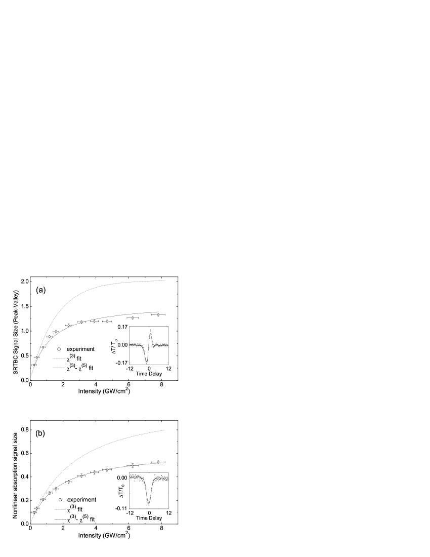
Figure 1: Intensity dependence of (a) SRTBC signal magnitude (normalized peak-valley transmission difference) and (b) nonlinear absorption signal of As₂S₃. The saturation of the cubic nonlinearity is evident. Higher-order nonlinearities, such as $\chi^{(5)}$, can be estimated from the deviation from $\chi^{(3)}$. Insets show examples of SRTBC and nonlinear absorption traces (symbols) along with the best-fit theoretical curves (solid lines). The time delay (on the horizontal axis) is given in units of the pulse duration (FWHM).

The dotted curves in both panels are predictions for the pure $\chi^{(3)}$ nonlinearity. The deviation of the experimental points from these curves evidences the saturation of the nonlinearity. Postulating the presence of the $\chi^{(5)}$ self-defocusing nonlinearity provides for good agreement with the experiments. Similar results were produced by all four samples used in the measurements; in particular, in all the cases the sign of the real part of $\chi^{(5)}$ turns out to be opposite to that of $\chi^{(3)}$, i.e., the quintic nonlinearity is self-defocusing indeed. The measured $\chi^{(3)}$ coefficients are consistent with previously reported values bala ; glassmeasurement_1 ; glass1 .

From these results, we also observe that higher-order nonlinearities become more important as the optical frequency approaches a resonance, as expected on physical grounds. The $\chi^{(5)}$ part of the nonlinearity is most significant for As₂S₃, while for sapphire it is below the detection threshold.

V Stability windows for the two- and three-dimensional solitons

The measurements provide the information needed to construct the window for the soliton formation. The results for 2D case are shown graphically in Fig. 2.

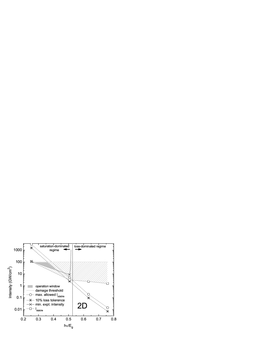
Figure 2: The operation window for the 2D solitons, as predicted on the basis of the experimentally-measured characteristics of the glass. The hatched area is the window neglecting the loss. The shaded area is the dramatically reduced (but definitely existing) window found with the loss taken into account.

The intensity limitations are plotted on the diagram against the reduced photon energy. The parameter space can be divided into two regions which were defined above, viz., the saturation-dominating and absorption-dominating ones, with the boundary between then determined by Eq. (12). To demonstrate the dramatic effect of the loss, we also plot the window for the (unrealistic) case when loss is completely neglected (the hatched area). In the absence of loss, the window is very large and the FOM increases monotonically with the reduced photon energy. The shaded area is the window remaining after inclusion of the loss. It is greatly reduced compared to the lossless case, and the best FOM is obtained near ${\hbar\omega}/{E_{g}}\simeq 0.35$. From this diagram, we conclude that, while the saturation of the nonlinearity is definitely necessary to stabilize the soliton, major restrictions on the window are imposed by the loss.

From the above rough estimation that were based on the band-edge arguments, one might expect that 3PA would further curtail the window, when the 2PA effects are weak (which is the case exactly inside the predicted window). However, $n_{2}$ and 2PA have been observed in glasses for the reduced photon energy as low as $\sim 0.35$ glass2 , due to the fact that the band edge in glasses extends well below the nominal value. Since significant 2PA remains in this region, 3PA may be neglected indeed. Hence, 2PA presents the fundamental limitation to observing solitons in these media [as quantified by the FOM in Eqs. (24) and (34)].

The results of the analysis for the 3D solitons are summarized in Fig. 3. Note that another major issue in this case is the requirement of anomalous GVD. This requirement is neglected here (addition of it will only further constrain the window, which does not really exist even without that, see below).

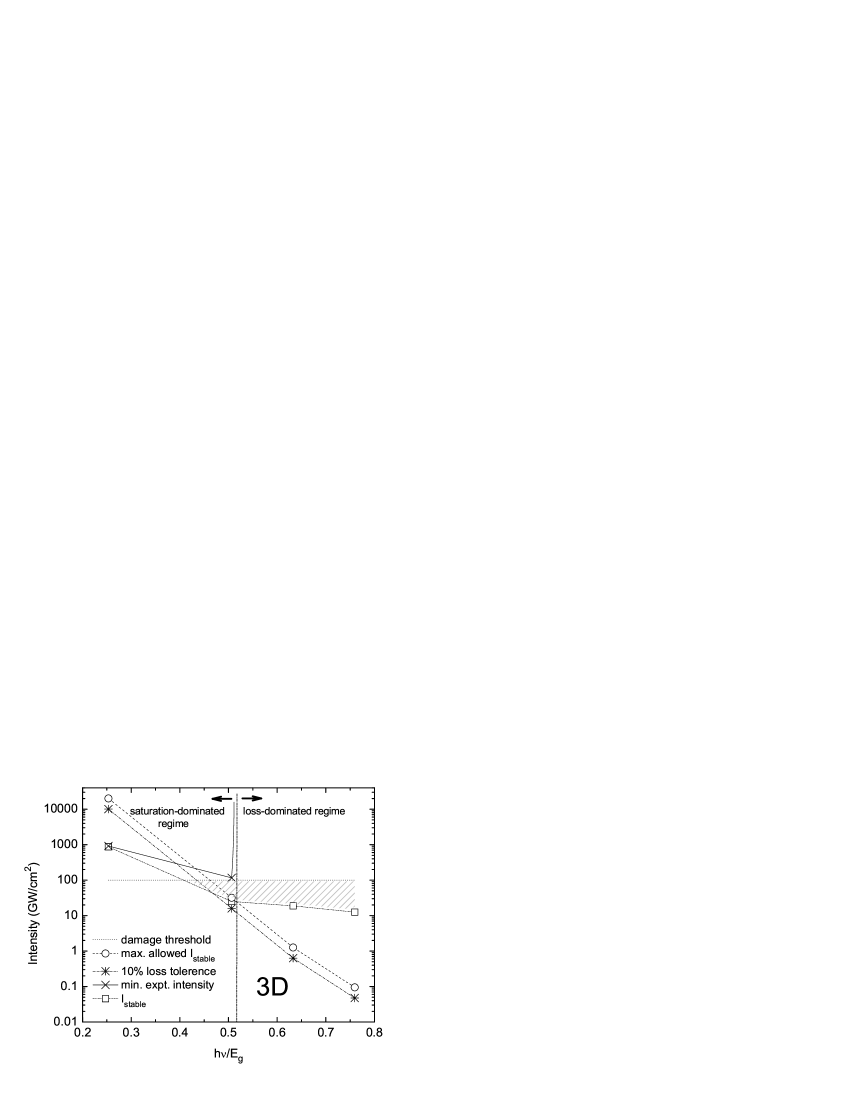
Figure 3: The operation window for 3D solitons. The meaning of the hatched area is the same as in the 2D case, i.e., it shows the window obtained neglecting the loss. When the loss is taken into account, the window vanishes completely.

From Fig. 3, we observe that, even in the lossless case, the window (hatched area) is significantly smaller than in the 2D case. This is expected, because collapse is stronger in 3D than 2D Luc . As in the 2D case, the loss again is a major concern for performing experiments. The most important inference is that the window closes up completely when loss is taken into account. Thus, it appears that loss will preclude the creation of 3D solitons in glasses, while leaving room for the 2D solitons.

Our overall conclusion is that a challenge is to perform experimental studies of 2D solitons in saturable Kerr media. Both spatial and spatiotemporal solitons are possible to be produced experimentally. Among these two, the 2D spatiotemporal case is more complicated since it requires anomalous GVD. In general, this will naturally constrain the window further. On the other hand, in this case tilted-pulse techniques could be used to obtain anomalous GVD. It is also possible to use a planar waveguide to perform 2D spatiotemporal soliton experiments.

Of course, the predicted window depends on the assumed parameters (such as the damage threshold) and criteria (such as the $10\%$ loss per diffraction length).Variations in these parameters will naturally impact the window, and our analysis provides the guidelines for searching for the most favorable materials and wavelength. A next natural step is to perform numerical simulations of the pulse propagation with the parameters selected in the present work. It is conceivable that the window for 3D solitons would finally open through variations of material parameters. In that case, one would still have to find an overlap of the resulting window with the condition that the GVD must be anomalous. More generally, non-glass materials may be tried to improve the possibilities for the experiment.

VI Conclusion

We have developed criteria for experimental observation of multi-dimensional solitons – spatial and spatiotemporal 2D solitons and spatiotemporal 3D ones. Using these criteria and measured properties of nonlinear glasses within a range of reduced photon energies, we have shown that the loss that accompanies higher-order nonlinearities (which are tantamount to saturation of the cubic nonlinearity) will set very stringent limits on the material parameters appropriate for the experiment. While loss was thus far neglected in theoretical treatments of multi-dimensional solitons, this work motivates more systematic studies of the soliton-like propagation in lossy media.
The criteria developed in this paper can also be applied, as an assessment tool, to materials other that glasses. More generally, the same rationale used for obtaining the relevant boundaries in this paper can also be used in systems other than optical ones. In these cases the specific mathematical forms of the boundaries will be different. In any case, the analysis presented here suggests that there is a small but apparently usable window of parameters in which 2D solitons can be generated, and work is underway to address this possibility. On the other hand, the prospects for generating 3D solitons in glasses are quite poor.

- (1) T. P. Stanton and L. A. Ostrovsky, Geophys. Res. Lett. 25, 2695 (1998).
- (2) S. Zhao, X. Xiong, F. Hu, and J. Zhu, Phys. Rev. E 64, 056621 (2001).
- (3) J. Schefer, M. Boehm, B. Roessli, G. A. Petrakovskii, B. Ouladdiaf, and U. Staub, Appl. Phys. A 74, s1740 (2002).
- (4) M. Hiraoka, H. Sakamoto, K. Mizoguchi, and R. Kato, Synth. Met. 133-134, 417 (2003).
- (5) L. Khaykovich, F. Schreck, G. Ferrari, T. Bourdel, J. Cubizolles, L. D. Carr, Y. Castin, and C. Salomon, Science 296, 1290 (2002).
- (6) P. K. Shukla, and F. Verheest, Astron. Astrophys. 401, 849 (2003).
- (7) I. Ballai, J. C. Thelen, and B. Roberts, Astron. Astrophys. 404, 701 (2003).
- (8) J. M. Ivanov, and L. V. Terentieva, Nucl. Phys. B, Proc. Suppl. 124, 148 (2003).
- (9) L. S. Brizhik, and A. A. Eremko, Electromagn. Biol. Med. 22, 31 (2003).
- (10) A. Wallraff, A. Lukashenko, J. Lisenfeld, A. Kemp, M. V.Fistul, Y. Koval, and A. V. Ustinov, Nature 425, 155 (2003).
- (11) G. P. Agrawal, Nonlinear Fiber Optics (Academic Press, San Diego, 1995).
- (12) J. McEntee, Fibre Systems Europe, January 2003, p. 19.
- (13) T. E. Bell, IEEE Spectr. 27, 56 (1990).
- (14) V. E. Zakharov and V. S. Synakh, Sov. Phys. JETP 41, 62 (1974).
- (15) Y. Silberberg, Opt. Lett. 15, 1282 (1990).
- (16) L. Bergé, Phys. Rep. 303, 260 (1998).
- (17) J. H. Marburger and E. Dawes, Phys. Rev. Lett. 21, 556 (1968).
- (18) P. M. Goorjian and Y. Silberberg, J. Opt. Soc. Am. B 14, 3253 (1997).
- (19) A. L. Dyshko, V. N. Lugovoi, and A. M. Prokhorov, Sov. Phys. JETP 34, 1235 (1972).
- (20) K. J. Blow and D. Wood, IEEE J. Quantum Electron. 25, 2665 (1989).
- (21) R. J. Hawkins and C. R. Menyuk, Opt. Lett. 18, 1999 (1993).
- (22) H. S. Eisenberg, R. Morandotti, Y. Silberberg, S. Bar-Ad, D. Ross D, and J. S. Aitchison, Phys. Rev. Lett. 87, 043902 (2001).
- (23) F. W. Wise, P. Di Trapani, Opt. Photonics News, 13, 28 (2002).
- (24) R. H. Enns, S. S. Rangnekar, and A. E. Kaplan, Phys. Rev. A 35, 466 (1987).
- (25) Y. Chen, Opt. Lett. 16, 4 (1991).
- (26) D.Edmundson, R. H. Enns, Opt. Lett. 17, 586 (1992).
- (27) D.Edmundson, R. H. Enns, Phys. Rev. A 51, 2491 (1995).
- (28) R. McLeod, K. Wagner, and S. Blair, Phys. Rev. A 52, 3254 (1995).
- (29) M. L. Quiroga-Teixeiro, A. Berntson, and H. Michinel, J. Opt. Soc. Am. B 16, 1697 (1999).
- (30) A. Desyatnikov, A. Maimistov, and B. Malomed, Phys. Rev. E 61, 3107 (2000).
- (31) B. A. Malomed, L.-C. Crasovan, and D. Mihalache, Physica D 161, 187 (2002).
- (32) M. Quiroga-Teixeiro and H. Michinel, J. Opt. Soc. Am. B 14, 2004 (1997).
- (33) I. Towers, A. V. Buryak, R. A. Sammut, B. A. Malomed, L. C. Crasovan, and D. Mihalache, Phys. Lett. A 288, 292 (2001); B. A. Malomed, L.-C. Crasovan, and D. Mihalache, Physica D 161, 187 (2002).
- (34) R. L. Pego and H. A. Warchall, J. Nonlinear Sci. 12, 347 (2002).
- (35) D. Mihalache, D. Mazilu, L.-C. Crasovan, I. Towers, A. V. Buryak, B. A. Malomed, L. Torner, J. P. Torres, and F. Lederer, Phys. Rev. Lett. 88, 073902 (2002).
- (36) J. E. Bjorkholm and A. Ashkin, Phys. Rev. Lett. 32, 129 (1974).
- (37) M. Segev, B. Crosignani, and A. Yariv, Phys. Rev. Lett. 68, 923 (1992).
- (38) G. C. Duree, Jr., J. L. Schultz, G. J. Salamo, M. Segev, A. Yariv, B. Crosignani, P. Di Porto, E. J. Sharp, and R. R. Neurgaonkar, Phys. Rev. Lett. 71, 533 (1993).
- (39) C. Etrich, F. Lederer, B. A. Malomed, T. Peschel, and U. Peschel, Progr. Optics 41, 483 (2000).
- (40) A. V. Buryak, P. Di Trapani, D. V. Skryabin, and S. Trillo, Phys. Rep. 370, 63 (2002).
- (41) W. E. Torruellas, Z. Wang, D. J. Hagan, E. W. VanStryland, G. I. Stegeman, L. Torner, and C. R. Menyuk, Phys. Rev. Lett. 74, 5036 (1995).
- (42) P. Di Trapani, D. Caironi, G. Valiulis, A. Dubietis, R. Danielius, and A. Piskarskas, Phys. Rev. Lett. 81, 570 (1998).
- (43) X. Liu, L. Qian, and F. W. Wise, Phys. Rev. Lett. 82, 4631 (1999).
- (44) X. Liu, K. Beckwitt, and F. W. Wise, Phys. Rev. E 62, 1328 (2000).
- (45) The influences of loss on one-dimensional spatial soliton formation and optical switch application in nonsaturable medium were considered in J. Bian and A. K. Chan, Micro. Opt. Technol. Lett. 5, 433 (1992), also see S. Blair, K. Wanger, and R. McLeod, J. Opt. Soc. Am. B 13, 2141 (1996).
- (46) A. Dubietis, E. Gaižauskas, G. Tamošauskas, and P. Di Trapani, Phys. Rev. Lett. 92, 253903 (2004).
- (47) M. A. Porras, A. Parola, D. Faccio, A. Dubietis, and P. Di Trapani, e-print physics/0404040.
- (48) I. Kang, T. D. Krauss, F. W. Wise, B. G. Aitken, and N. F. Borrelli, J. Opt. Soc. Am. B 12, 2053 (1995).
- (49) J. M. Harbold, F. O. Ilday, F. W. Wise, J. S. Sanghera, V. Q. Nguyen, L. B. Shaw, and I. D. Aggarwal, Opt. Lett. 27, 119 (2002).
- (50) J. M. Harbold, F. O. Ilday, F. W. Wise, and B. G. Aitken, IEEE Photon. Tech. Lett. 14, 822 (2002).
- (51) F. Smektala, C. Quemard, V. Couderc and A. Barthélémy, J. Non-Cryst. Sol. 274, 232 (2000).
- (52) I. Kang, T. Krauss, and F. W. Wise, Opt. Lett. 22, 1077 (1997).
- (53) Y.-F. Chen, K. Beckwitt, and F. W. Wise (in preparation).
- (54) D. W. Hall, M. A. Newhouse, N. F. Borrelli, W. H. Dumbaugh, and D. L. Weidman, Appl. Phys. Lett. 54, 1293 (1989).
- (55) V. E. Zakharov and A. M. Rubenchik, Sov. Phys. JETP 38, 494 (1974).