Lifetime and hyperfine splitting measurements on the $7s$ and $6p$ levels in Rb

Abstract

We present lifetime measurements of the $7S_{1/2}$ level and the $6p$ manifold of Rb. We use a time-correlated single-photon counting technique on a sample of ⁸⁵Rb atoms confined and cooled in a magneto-optical trap. The upper state of the $5P_{1/2}$ repumping transition serves as the resonant intermediate level for two-photon excitation of the $7s$ level. A probe laser provides the second step of the excitation, and we detect the decay of the atomic fluorescence to the $5P_{3/2}$ level at 741 nm. The decay process feeds the $6p$ manifold which decays to the $5s$ ground state emitting uv photons. We measure lifetimes of $88.07\pm 0.40$ ns and $120.7\pm 1.2$ ns for the $7S_{1/2}$ level and $6p$ manifold, respectively; while the hyperfine splitting of the $7S_{1/2}$ level is $282.6\pm 1.6$ MHz. The agreement with theoretical calculations confirms the understanding of the wavefunctions involved, and provides confidence on the possibility of extracting weak interaction constants from a Parity Non-Conservation measurement.

I Introduction

The lifetime of an excited level and its hyperfine splitting are properties related to the electronic wavefunctions of the atom. The lifetime, through the matrix elements of allowed transitions, probes the wavefunctions at large radius, while the hyperfine splitting samples their value at the nucleus. The comparison of the two types of measurements with theoretical predictions test the quality of the computed wavefunctions. The calculation of the wavefunctions have now reached new levels of sophistication johnson03 ; flambaum04 based on Many Body Perturbation Theory (MBPT). Those calculations are particularly important in the interpretation of precision tests of discrete symmetries in atoms: Parity Non-Conservation (PNC) (see for example the Cs measurements of Wood et al. wood97 ; wood99 ) and Time Reversal (TR).lamoreaux

This paper presents our measurements on ⁸⁵Rb atoms in a magneto-optic trap (MOT) using time-correlated single-photon counting techniques. We measure the lifetimes of the $7s~{}^{2}S_{1/2}$ level and the $6p$ manifold as well as the hyperfine splitting of the $7s~{}^{2}S_{1/2}$ level. The work complements and aids our program of Fr spectroscopy and weak interaction physics.orozco02 We carry out all the Fr measurements in a trapped and cooled atomic gas. Rb and Fr have very similar properties and the same trap can be used to capture either of them by selecting the appropriate wavelengths.aubin03a Having the ability to trap both atoms helps us understand better our experimental results. The trap is optimized for Fr and it works on-line with the Superconducting LINAC at Stony Brook. Our Rb measurements are necessary to fully understand the systematic effects on our measurements of the equivalent levels in Fr, $9s,8p$.aubin03b ; aubin04

The Rb measurements presented here are an important test of MBPT calculations in a regime where relativistic effects are not as important as in heavier atoms such as Fr. Measurements of excited state atomic lifetimes in the low-lying states of the $s$ and $p$ manifolds enhance our understanding of the wavefunctions and the importance of correlation corrections in their calculation.

The paper is structured as follows: We present the lifetime measurements in section II, detail the hyperfine splitting measurement in section III, and summarize the work in the context of similar measurements in Rb and Fr in section IV.

II Lifetime measurements

II.1 Lifetime and matrix elements

The lifetime of a quantum mechanical system depends on the initial and final states wavefunctions and the dominant interaction. Since the electromagnetic interaction in atomic physics is well understood, radiative lifetimes provide information on atomic structure.

The lifetime $\tau$ of an excited state is related to the partial lifetimes $\tau_{i}$ associated with each of the allowed decay channels by:

$$1/\tau=\sum_{i}1/\tau_{i}.$$ (1)

The matrix element associated with a partial lifetime between two states connected with an allowed dipole transition is given by:cowan

$$\frac{1}{\tau_{i}}=\frac{4}{3}\frac{\omega^{3}}{c^{2}}\alpha\frac{|\langle J\|r\|J^{\prime}\rangle|^{2}}{2J^{\prime}+1},$$ (2)

where $\omega$ is the transition energy divided by $\hbar$, $c$ is the speed of light, $\alpha$ is the fine-structure constant, $J^{\prime}$ and $J$ are respectively, the initial and final state angular momenta, $\tau_{i}$ is the excited state partial lifetime, and $|\langle J\|r\|J^{\prime}\rangle|$ is the reduced matrix element.

The calculation of the radial matrix elements requires the wavefunctions of the initial and final states involved in the decay. The contributions of the wavefunction at large distance become more important due to the presence of the radial operator. Knowledge of the atomic lifetimes and branching ratios in Rb will determine the radial matrix elements for the transitions.

II.2 Sample preparation

We use a high efficiency magneto-optical trap (MOT) to capture a sample of Rb atoms at a temperature lower than 300 $\mu$K.aubin03a We load the MOT from a Rb vapor produced by a dispenser in a glass cell coated with a dry film. The MOT consists of three pairs of retro-reflected beams, each with 15 mW/cm² intensity, 6 cm diameter (1/e² intensity) and red detuned 19 MHz from the atomic resonance. A pair of coil generates a magnetic field gradient of 6 G/cm. We trap 10⁵ atoms, with a diameter of 0.2 mm and a typical lifetime between 5 and 10 s.

Figure 1 shows the energy levels of ⁸⁵Rb relevant for the trap, lifetime and hyperfine splitting measurements. The trapping and cooling are done with a Coherent 899-21 titanium-sapphire (ti-sapph) laser at 780 nm between the $5S_{1/2}$ $F=3$ and the $5P_{3/2}$ $F=4$ levels. We repump the atoms that fall out of the cycling transition with a Coherent 899-01 ti-sapph laser at 795 nm between the $5S_{1/2}$ $F=2$ and the $5P_{1/2}$ $F=3$ levels. A Coherent 899-21 ti-sapph at 728 nm, the probe laser, completes the two photon transition. We use a depumper pulse at 780 nm between the $5S_{1/2}$ $F=3$ and the $5P_{3/2}$ $F=3$ levels before the two photon transition to take the atoms out of the cycling transition and into the lower hyperfine ground state.

The atoms in the trap are excited to the $7s$ level using a two photon transition through the $5P_{1/2}$ level. To increase the population transfer to the $7s$ level we split the repumper light into two paths, one going directly to the trap with a large beam size to optimize the trapping efficiency and combining the other with the depumper and probe laser focused on the trap to optimize the excitation. We send 12 mW of probe power, 9 $\mu$W of depumper power and 2 mW of repumper power focused to a spot size between 1 and 3 mm to increase the excitation intensity.

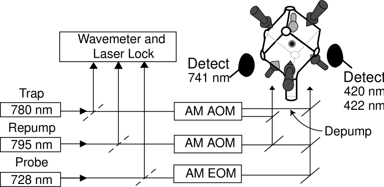
Figure 2: Schematic of the trap. AM EOM stands for amplitude modulation with an electro-optic modulator and AM AOM for amplitude modulation with an acousto-optic modulator. gomezF2.EPS.

Figure 2 shows the schematic of the laser system. We control the power of the lasers going into the trap with acousto-optic modulators (AOM) and electro-optic modulators (EOM). We measure the wavelength of the lasers with a wavemeter (Burleigh WV-1500). We lock the trap laser to ⁸⁵Rb using saturation spectroscopy. We avoid long term frequency drifts on the probe and repumper lasers by transferring the long term stability of a He-Ne laser to the two lasers via a computer controlled scanning Fabry-Perot cavity.zhao98

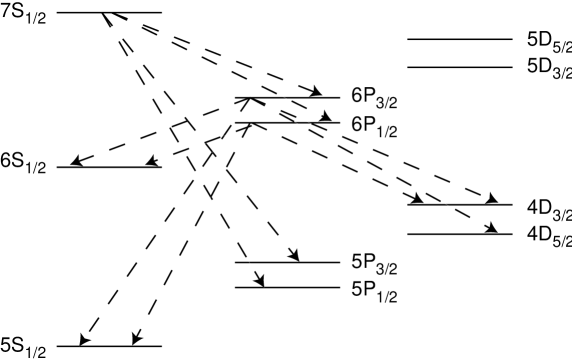
Figure 3: Decay paths for the $7s$ and $6p$ levels of ⁸⁵Rb. gomezF3.EPS.

The $7s$ level has four different electric dipole (E1) allowed decay channels as shown in Fig. 3. We detect the direct decay channel from the $7s$ to the $5P_{3/2}$ at 741 nm to obtain the lifetime of the $7s$ level. The $7s$ level can also decay to the $6p$ level and from there cascade down to the $5s$ level emitting a photon at 420 (or 422) nm in this last step. We collect the fluorescence at 420 (or 422) nm that contains contributions from the lifetime of the $7s$ and $6p$ levels. Using the results obtained for the lifetime of the $7s$ level we can extract a lifetime for the $6p$ manifold.

II.3 Experimental method

We use the technique of time-correlated single-photon counting to measure the lifetimes.oconnor84 This method has been used in the past to measure lifetimes of atoms in beams,young94 vapor cellshoeling96 and single ions.devoe94 Our group has used it to measure the lifetime of the $7p$, $7d$ and $9s$ levels in Fraubin03b ; aubin04 ; simsarian98 ; grossman00b and of the $5p$ levels in Rb.simsarian98

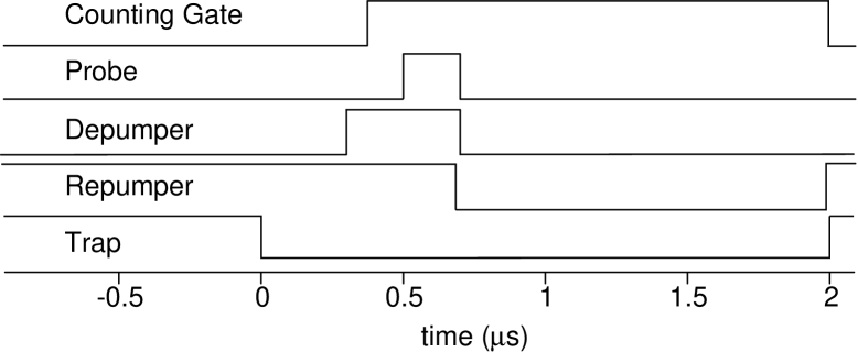
Figure 4: Timing sequence for the excitation of atoms to the $7s$ level. High level is on, low level is off. gomezF4.EPS.

The cycle of the measurement has a repetition rate of 100 kHz controlled with a Berkeley Nucleonics Corporation BNC 8010 pulse generator and two Stanford Research Systems DG535 pulse delay generators as shown in Fig. 4. The cycle starts with 0.7 $\mu$s for state preparation. To do this we first take the atoms out of the cycling transition and into the lower hyperfine ground level with a depumper beam at 780 nm between the $5S_{1/2}$ $F=3$ and the $5P_{3/2}$ $F=3$ level, (a) in Fig. 1. Once there, the atoms are excited with the repumper laser to the $5P_{1/2}$ $F=3$ level, (b) in Fig. 1, and from there the probe laser takes them to the $7S_{1/2}$ $F=3$ level, (c) in Fig. 1. We detect fluorescence for 1.6 $\mu$s while the counting gate is on while keeping all the lasers off during the last 1.3 $\mu$s. We use the rest of the cycle (8 $\mu$s) for cooling and trapping of atoms. At the beginning of the cycle we turn off the trap laser with an acousto-optic modulator (AOM)(Crystal Technology 3200-144). The trap beam is focused to a transverse line in the AOM with a cylindrical lens telescope to avoid damage to the crystal while maintaining a large diffraction efficiency. This gives a 10:1 on/off ratio for the trap laser in 260 ns. We allow an extra 240 ns to increase the on/off ratio for the trap laser before we excite the atoms to the $7s$ level for 200 ns. We turn off the probe with two electro-optic modulators (EOM)(Gs${\rm\ddot{a}}$nger LM0202) and an AOM (Crystal Technology 3200-144). The two EOM’s give a fast turn off for the probe laser and the AOM improves the long term on/off ratio. The turn off of the probe laser can be approximated with a half Gaussian function with a FWHM of 7 ns. We obtain an on/off ratio of 600:1 after 20 ns. The fast turn off of the EOM’s creates strong radio frequency (RF) emission. The photomultiplier tube (PMT) amplifiers can pick this emission and create false detection pulses. We minimize these false events by enclosing the EOMs and drivers inside a metallic cage in a separate room. Another AOM (Crystal Technologies 3200-144) turns off the repumper simultaneously with the probe. We look for fluorescence from the $7s$ level and the $6p$ manifold for 1.3 $\mu$s. We turn the trapping beams back on for the rest of the cycle and then repeat the entire cycle continuously for the duration of the measurement.

A 1:1 imaging system (f/3.9) collects the fluorescence photons onto a charge coupled device (CCD) camera (Roper Scientific, MicroMax 1300YHS-DIF). We monitor the trap with the use of an interference filter at 780 nm in front of the camera. A beam-splitter in the imaging system sends 50$\%$ of the light onto a PMT (Hamamatsu R636). An interference filter at 741 nm in front of the PMT reduces the background light other than fluorescence from the $7S_{1/2}$ to the $5P_{3/2}$ level. Another independent 1:1 imaging system (f/3.5) monitors the fluorescence from the $6p$ manifold to the $5S_{1/2}$ level with the use of an interference filter at 420 nm (10 nm bandwidth at 50$\%$) and a PMT (Amperex XP 2020Q).

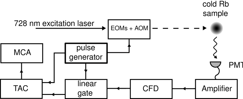
Figure 5: Block diagram for the electronics used for the detection of $7s$ or $6p$ photons. gomezF5.EPS.

Figure 5 shows a block diagram of the electronics used in the detection and processing of $7s$ and $6p$ photon events. The heart of the electronics is the time-to-amplitude converter (TAC) (Ortec 467 for the $7s$ photons and Ortec 437 for the $6p$ photons). The TAC receives an start and an stop pulse and outputs a voltage proportional to the time separation between pulses. The pulse generator used to control the timing of the lasers provides the stop pulse at a fixed delay from the lasers turn off. A detected fluorescence photon provides the start pulse. Only one photon can be processed per cycle. The photon pulse generated by the PMT goes through some processing before reaching the TAC. It first goes through an Ortec AN106/N amplifier and then to an Ortec 934 constant fraction discriminator (CFD). The output of the discriminator is a pulse of fixed shape with a constant time delay from the input pulse. The pulse then goes through a linear gate (Ortec LG101/N) which is open only during the excitation and fluorescence part of the cycle. Starting the TAC with a fluorescence photon eliminates the cycles with no detected photons. An histogram of the output of the TAC in a multichannel analyzer (MCA) (EG$\&$G Trump-8k for the $7s$ photons and Canberra 3502 for the $6p$ photons) displays the exponential decay directly in real-time.

We calibrate the MCA by replacing the start pulse given by the PMT with an electronic pulse generated by the pulse generator. We change the separation between the start and stop pulses in steps of 100 ns and fit the resulting signal to find both the linearity and calibration. We verify the uniformity of the MCA channels by triggering the PMT with random photon events from room light. The result is a uniformly flat signal consistent with zero slope.

II.4 $7s$ level analysis

We measure the lifetime of the $7s$ level through its decay to the $5P_{3/2}$ level. We keep the number of atoms in the trap low (about 10⁵) to reduce density related effects (diameter of the trap $\sim$ 0.2 mm). We operate with the number of detected photons per cycle to be much smaller than one. We apply a small correction to the data to account for preferential counting of early events.oconnor84 This correction appears when we have more than one photon per cycle. The correction, called pulse pileup correction, is given by

$${\cal N}^{\prime}_{i}=\frac{{\cal N}_{i}}{1-\frac{1}{n_{E}}\sum_{j<i}{\cal N}_{j}},$$ (3)

where ${\cal N}_{i}$ is the number of counts in channel $i$ of the MCA, $n_{E}$ is the total number of cycles, and ${\cal N}^{\prime}_{i}$ is the corrected number of counts for channel $i$. We typically get one count every 100 cycles (or 1 ms), which corresponds to a correction smaller than 1$\%$ in the number of counts per channel.

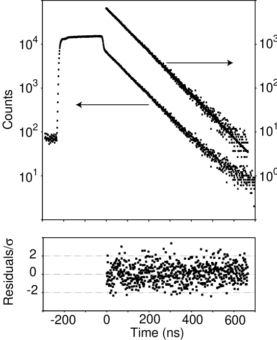
Figure 6: Exponential decay of the $7s$ level. The upper plot contains the raw data that shows the excitation turn on and turn off as well as the exponential decay of the atoms (left scale). It also shows the background subtracted signal together with the exponential fit (right scale). The lower plot shows the normalized residuals (assuming statistical noise). gomezF6.EPS.

Figure 6 shows the exponential decay obtained for a 47 minute accumulation along with the fit and residuals. For times before -200 ns the small signal comes from the trapping laser light leakage through the interference filter. Between t=-200 ns and t=0 ns we turn on the excitation beams (probe and depumper) which gives the fast rise and plateau on the signal coming both from the fuorescence of the atoms and the leakage from the two additional lasers, after t=0 ns we turn all the laser beams off and the only light remaining is the fuorescence from the atoms. The fit starts 20 ns after the beams turn off and stops when the signal is equal to the background. The fitting function is

$$S_{7s}=c_{a}e^{-t/\tau}+c_{b}+c_{m}t,$$ (4)

with $t$ the time (or channel number) and $\tau$ and $c_{i}$ ($i=a,b,m$) the fitting constants. We obtain a background signal by repeating the experiment without atoms. The lifetime fit is affected slightly by the presence of a linear background that we include in the fit. The slope of the background is about 2 counts per 1000 channels per 1000 seconds of accumulation and comes from the slow turn off of the trap laser. This particular decay has a reduced $\chi^{2}_{\nu}$ of 1.07, where the noise in the number of counts is statistical ($\sqrt{S}$). A discrete Fourier transform of the residuals shows no structure.

II.4.1 Systematic effects

We search for systematic effects by varying one experimental parameter at a time and looking for an effect on the obtained lifetime. Each measurement lasts for about 3000 s. We study first the effects that the external variables have on the lifetime. Each measurement is obtained under slightly different conditions. We fit them independently using the fitting function of Eq. 4 and make a correlation study between the obtained lifetime and the external variable for each case.

Excitation pulse duration. We change the excitation pulse duration between 100 and 800 ns. The lifetime is independent of the initial conditions of the decay. Changing the pulse duration can modify the initial conditions for the decay.

Probe intensity. We vary the probe intensity over a factor of ten. This is another way in which we can modify the initial conditions for the decay.

Magnetic field. The presence of a magnetic field from the MOT may influence the measured lifetime mainly through quantum beats between the Zeeman sublevels. We change the magnetic field gradient from 4 to 7 Gauss/cm.

Number of atoms. We change the number of atoms from 6$\times$10⁴ to 1$\times$10⁷. Increasing the number of atoms will increase the density and produce more collisions between the atoms as well as permit radiation trapping. These two effects will modify the lifetime. The photon detection rate also increases with the atom number. This rate becomes too high for the electronics of the MCA and the repetition rate for the experiment has to be reduced to 10 kHz, with a larger pulse pile-up correction.

We quantify the correlation between the measured lifetime and the external variables by calculating the linear correlation coefficient. The integral of the probability distribution associated with the linear correlation coefficient provides the degree of correlation of the data with the external variable. An small value for the integral probability means significant correlation. In all of the above cases the integral probability of the linear correlation coefficient is larger than 5$\%$, consistent with no correlation. We keep the number of atoms low for all the measurements to avoid systematic effects related to collisions or to pulse pile-up. Radiation trapping can be ignored due to the small population in the $5P_{3/2}$ level.

Other effects can influence the measurement but they are not related to a simple variable as above. In this case we make a reference measurement and then we modify something to test each one of the above potential effects to obtain another measurement. We fit each independent data file using Eq. 4 and perform an $\chi^{2}$ test to the obtained lifetimes to find out if they are consistent with statistical fluctuations.

Repumper turn off. We look for an effect of an imperfect turn off of the repumper light by leaving the repumper on continuously. The repumper is used as the first step of the two photon transition and when combined with an imperfect turn-off of the probe laser it can introduce a false signal.

Hyperfine level. To our accuracy level, the lifetime should be independent of the hyperfine level. We change the initial hyperfine level of the decay, that is, instead of preparing the atoms in the $7S_{1/2}$ $F=3$ state we prepare them in the $7S_{1/2}$ $F=2$ state.

Electronics. We look for effects related to the electronic components by interchanging the MCA for the $7s$ and $6p$ detection systems. It is important to keep the Canberra MCA count rate low.

Probe turn off. An imperfect extinction of the probe laser will show up as an excess in the initial data points of the decay. This effect can be revealed by changing the initial/final point for the fit. The spread of the lifetimes as a function of the starting point of the fit is consistent with the statistical uncertainty. There is no dependence on the final point for the fit within our statistical precision.

All the above measurements give an integral probability for the $\chi^{2}$ between 5$\%$ and 95$\%$, consistent with statistical fluctuations.

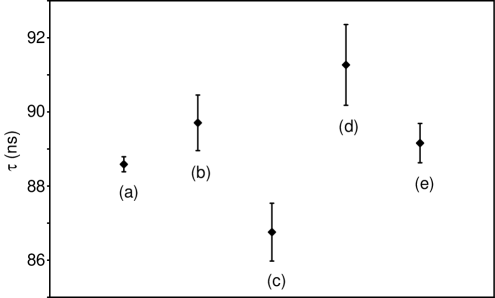
Figure 7: Lifetime obtained when the trap is displaced by inserting a piece of glass in the retro-reflection mirrors of the MOT while the magnetic field environment remains unchanged. (a) no displacement, (b) displacement using mirror 1, (c) mirror 2, (d) mirror 3 and beams realigned, (e) no displacement and beams not realigned. gomezF7.EPS.

Trap displacement. We displace the trap keeping the magnetic field fixed, such that the atoms are sampling a different magnetic environment. To move the trap position we insert a piece of glass in front of one of the retro-reflection mirrors in the MOT. We repeat the same procedure for the three retro-reflection mirrors in the MOT. The MOT image on the camera shows trap displacements smaller than one trap diameter in the transversal direction to the camera and we have no information on the longitudinal displacement. This is a complex systematic effect since it involves the change of several experimental parameters such as the alignment of the excitation lasers. This makes it difficult to assign a single parameter responsible for the variations we observe. We tried different combinations of moving the trap with and without realignment. The integral probability of the $\chi^{2}$ shows fluctuations larger than statistical. We include an uncertainty contribution of $\pm$0.38$\%$, equal to the dispersion of the lifetime values (Fig. 7).

Quantum beats. We look for quantum beats in the residuals of the fit. A discrete Fourier transform of the residuals shows no structure. The value of $\pm$0.1$\%$ quoted for the uncertainty due to quantum beats comes from a theoretical calculation with a simple model which assumes well defined Zeeman sublevels as in the presence of a uniform magnetic field. The presence of a magnetic field gradient further reduces the quantum beat contribution.

Some of the information obtained can be extended to measurements in Fr. Changing the number of atoms is complicated in Fr so we can use the results for Rb to know if we are working in a good regime. Both atoms have similar atomic structure, so most tests should give similar results. The most important difference is their sensitivity to magnetic effects because of the difference in multiplicity of Zeeman sublevels and hyperfine separation.

II.4.2 Result and comparison with theory

The average of the reduced $\chi_{\nu}^{2}$ of the individual files is 1.04$\pm$0.08. The different lifetimes from the fit are averaged to obtain the final result. The lifetime of the $7s$ level is 88.07$\pm$0.38 ns. A fit to the file resulting from adding all the files gives consistent results. Table 1 summarizes the error budget for the experiment.

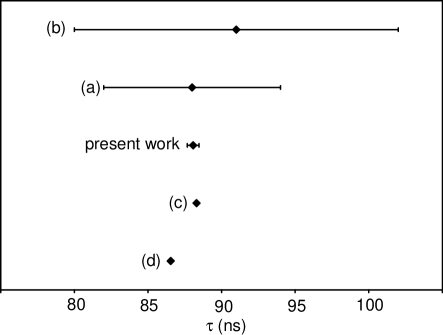
Figure 8: Experimental result of the 7s lifetime in Rb, together with previous experimental results: (a)Marek et al,marek80 (b)Bulos et al,bulos76 and theoretical predictions: (c)Safronova et al,safronova03 (d)Theodosiou.theodosiou84 gomezF8.EPS.

Figure 8 is a comparison of our result with theoretical predictionssafronova03 ; theodosiou84 for the lifetime of the $7s$ level, as well as previous measurements.marek80 ; bulos76 Theoretical calculations are reaching a level of precision below 1$\%$.derevianko01 An experimental verification of this precision is important to increase the confidence in such calculations. This information is crucial to extract weak interaction physics out of parity non-conservation experiments. The prediction from ab initio calculations for the $7s$ level lifetime is 88.3 ns.safronova03 The agreement shows the remarkable level of sophistication of atomic structure calculations.

II.5 $6p$ level analysis

The $7s$ level has the four decay channels shown in Fig. 3. We detect the indirect decay from the $6p$ to the $5s$ levels to obtain information about the $6p$ level. The atoms decaying from the $6p$ level come from a cascade decay from the $7s$ level and the decay cannot be described with a single exponential. The signal from this indirect decay is the sum of three exponential functions with lifetimes corresponding to the $7S_{1/2}$, $6P_{1/2}$ and $6P_{3/2}$ levels. We can make use of the result obtained in the previous section for the lifetime of the $7S_{1/2}$ level to measure the lifetime of the $6p$ manifold. Here we present the analysis of the $6p$ signal that contains contributions from the two fine levels. The fine separation of the $6p$ levels in Rb is 1.4 nm which is smaller than the 10 nm transmission width of the interference filter. In the case of Fr, the fine separation of the corresponding levels is larger and we use interference filters to resolve both contributions seperately.aubin03b ; aubin04

The lifetimes of the two fine $6p$ levels are expected to be similar. We assume that the decay signal is given by the sum of two exponential functions, one for the $7s$ level and the other for the $6p$ level, so that the fitting function is

$$S_{6p}=A_{b}+A_{7s}e^{-t/\tau_{7s}}+A_{6p}e^{-t/\tau_{6p}},$$ (5)

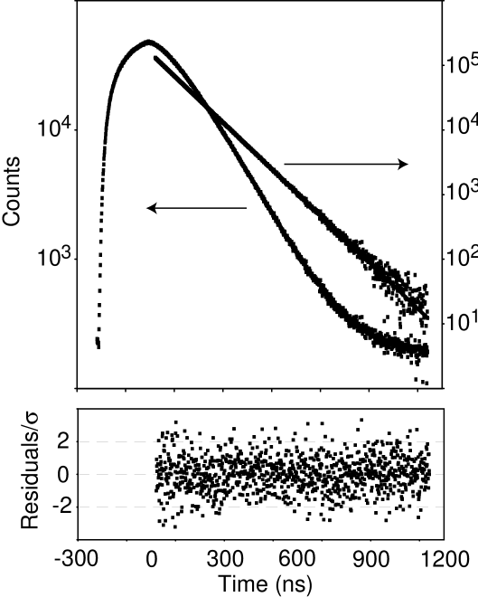
Figure 9: Decay of the $6p$ manifold. The upper plot contains the raw data (left scale) and the data minus the background minus the exponential contribution from the $7s$ level (right scale). An exponential fit to this last curve is also shown. The lower plot contains the normalized residuals (assuming statistical noise). gomezF9.EPS.

where $\tau_{7s}$ is the lifetime of the $7s$ level obtained in the previous section, and $\tau_{6p},A_{b},A_{7s}$ and $A_{6p}$ are the fitting constants. Fig. 9 shows the signal obtained for a single file and the resulting curve if we subtract the background and the exponential contribution from the $7s$ level. This last curve corresponds to the exponential decay of the $6p$ manifold. We only use files with low count rates to avoid systematic effects associated with the slow response of the MCA.

The lifetime we obtain for the $6p$ manifold depends on the value of the lifetime of the $7s$ level. The uncertainty in the $7s$ lifetime influences the precision with which we can extract the $6p$ lifetime. The probability distribution for $\tau_{6p}$ is given by

$$P(\tau^{\prime\prime})=\int d\tau^{\prime}\frac{1}{\sqrt{2\pi}\sigma_{7s}}e^{-\frac{1}{2}\left(\frac{\tau^{\prime}-\tau_{7s}}{\sigma_{7s}}\right)^{2}}\frac{1}{\sqrt{2\pi}\sigma_{6p}(\tau^{\prime})}e^{-\frac{1}{2}\left(\frac{\tau^{\prime\prime}-\tau_{6p}(\tau^{\prime})}{\sigma_{6p}(\tau^{\prime})}\right)^{2}}.$$ (6)

The integrand contains two Gaussian distributions, the first one gives the probability distribution for $7s$ level lifetime centered on $\tau_{7s}$ with an uncertainty $\sigma_{7s}$ and the second one gives the probability distribution for the $6p$ manifold lifetime centered on $\tau_{6p}(\tau^{\prime})$ with an uncertainty $\sigma_{6p}(\tau^{\prime})$. We assume a value $\tau^{\prime}$ for the lifetime of $\tau_{7s}$ and include that in the fitting function (Eq. 5) to obtain a value for $\tau_{6p}(\tau^{\prime})$. We repeat the same procedure for different values of $\tau^{\prime}$ and perform the integral of Eq. 6.

The result for the integral when $\tau_{6p}$ and $\sigma_{6p}$ do not strongly depend on $\tau^{\prime}$ gives approximately $\tau_{6p}=\tau_{6p}(\tau_{7s})=120.7$ ns and $\sigma_{6p}=\sqrt{\sigma_{6p}(\tau_{7s})^{2}+\left(\frac{d\tau_{6p}(\tau^{\prime})}{d\tau^{\prime}}\sigma_{7s}\right)^{2}}=0.35$ ns, as confirmed by numerical integration. This result assumes uncorrelated errors for the individual files used on the fit but includes the spread brought by systematic checks on the $7s$ level lifetime. The uncertainty in the MCA calibration is at the 0.94$\%$ level. Table 2 summarizes the error budget that gives a final result for the lifetime of the $6p$ manifold of 120.7$\pm$1.2 ns.

II.5.1 Simple model

We can make a comparison between the predicted and the measured signal to give some bounds on the possible values for the lifetime of each fine level.

The decay signal is obtained by solving the following rate equations

$$\frac{dN_{s}}{dt}=-\frac{N_{s}}{\tau_{s}},$$

$$\frac{dN_{p1}}{dt}=B_{p1}\frac{N_{s}}{\tau_{s}}-\frac{N_{p1}}{\tau_{p1}},$$

$$\frac{dN_{p3}}{dt}=B_{p3}\frac{N_{s}}{\tau_{s}}-\frac{N_{p3}}{\tau_{p3}},$$ (7)

where $N_{i}$ and $\tau_{i}$ give the population and lifetime respectively of level $i$, with $i=s,p1,p3$ representing the $7S_{1/2}$, $6P_{1/2}$ and $6P_{3/2}$ levels, and $B_{p1}=0.132,B_{p3}=0.255$ the theoretical branching ratios from the $7S_{1/2}$ level to the $6P_{1/2}$ and $6P_{3/2}$ respectively.safronova03 To solve this equations we need the initial conditions for the level populations at the beginning of the decay (or equivalently at the end of the excitation pulse). Fig. 6 shows that during the excitation the population of the $7s$ level reaches an steady state very fast. We will assume the $7s$ population to be constant during the excitation pulse. We also assume that before the excitation we have no population in the $6p$ level. With these assumptions we can calculate the population of the $6p$ levels during the excitation given by

$$N_{p1}=N_{s}B_{p1}\frac{\tau_{p1}}{\tau_{s}}(1-e^{-t/\tau_{p1}}),$$

$$N_{p3}=N_{s}B_{p3}\frac{\tau_{p3}}{\tau_{s}}(1-e^{-t/\tau_{p3}}).$$ (8)

The excitation lasts for $T$=200 ns, so evaluating these expressions after this time will give the initial conditions for the decay. Solving Eq. 7 with these initial conditions gives the population of the three levels as a function of time. The signal measured by the PMT is proportional to the sum of the decay rates of each of the $6p$ levels to the $5s$ level. The underlying assumption that the response of the PMT and the interference filter is the same for both of the $6p$ levels is reasonable due to the small energy separation between them (1.4 nm). The signal ($\widetilde{S_{6p}}$) coming out of the PMT is given by

$$\widetilde{S_{6p}} =\widetilde{A_{b}}+\widetilde{A}\left(b_{p1}\frac{N_{p1}}{\tau_{p1}}+b_{p3}\frac{N_{p3}}{\tau_{p3}}\right),$$ (9)

$$=\widetilde{A_{b}}+\widetilde{A^{\prime}}\left[\left(\frac{b_{p1}B_{p1}}{\tau_{s}-\tau_{p1}}+\frac{b_{p3}B_{p3}}{\tau_{s}-\tau_{p3}}\right)e^{-t/\tau_{s}}+b_{p1}B_{p1}\left(\frac{1-e^{-T/\tau_{p1}}}{\tau_{s}}-\frac{1}{\tau_{s}-\tau_{p1}}\right)e^{-t/\tau_{p1}}\right.$$

$$\left.+b_{p3}B_{p3}\left(\frac{1-e^{-T/\tau_{p3}}}{\tau_{s}}-\frac{1}{\tau_{s}-\tau_{p3}}\right)e^{-t/\tau_{p3}}\right],$$

where $b_{p1}=0.194,b_{p3}=0.236$ are the branching ratios for the decays from the $6P_{1/2}$ and $6P_{3/2}$ to the $5s$ level respectivelysafronova03 and $\widetilde{A_{b}},\widetilde{A}$ and $\widetilde{A^{\prime}}$ the background and scale constants.

To compare this expression with Eq. 5 we need to combine the two exponential functions for the $6p$ levels into a single one since we do not have enough resolution to separate them, that is we need to make

$$b_{p1}B_{p1}\left(\frac{1-e^{-T/\tau_{p1}}}{\tau_{s}}-\frac{1}{\tau_{s}-\tau_{p1}}\right)e^{-t/\tau_{p1}}+b_{p3}B_{p3}\left(\frac{1-e^{-T/\tau_{p3}}}{\tau_{s}}-\frac{1}{\tau_{s}-\tau_{p3}}\right)e^{-t/\tau_{p3}}\sim Ce^{-t/\tau^{\prime}_{6p}}.$$ (10)

The two expressions above will be equal in the least squares sense, meaning that we will solve for the values of C and $\tau^{\prime}_{6p}$ that minimize the square of the difference of the two sides of the equation in the range from 0 to $\infty$. The theoretical values for the $6p$ fine level lifetimes are $\tau_{p1}=129$ ns, $\tau_{p3}=118$ ns.safronova03 Using these values we get the following expression for the signal

$$\widetilde{S_{6p}}=\widetilde{A_{b}}+\widetilde{C}(e^{-t/\tau_{s}}-1.29e^{-t/\tau^{\prime}_{6p}}),$$ (11)

with $\tau^{\prime}_{6p}=120.7ns$. The ratio of the amplitudes of the $7s$ and $6p$ exponential functions is fixed by this model. Using the fitting parameters from Eq. 5 for the experimental result we obtain $A_{6p}/A_{7s}=-1.44\pm 0.01$. The difference between the predicted ratio and the one obtained is 12$\%$.

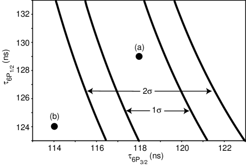
Figure 10: Constraints on the lifetimes of the two $6p$ fine levels in Rb using the model described in the text and the experimental result. The solid lines define the limits of the 1$\sigma$ and 2$\sigma$ regions respectively. The circles are theoretical predictions: (a)Safronova et al,safronova03 (b)Theodosiou.theodosiou84 gomezF10.EPS.

We can invert the previous procedure to set limits on the possible values of the $6p$ fine level lifetimes. If we take $\tau^{\prime}_{6p}$ equal to the experimental value (or some other value) we can only obtain that value with specific combinations of $\tau_{p1}$ and $\tau_{p3}$. This will not fix either $\tau_{p1}$ or $\tau_{p3}$, but it will create a functional relation between the two. Fig. 10 gives the 1$\sigma$ and 2$\sigma$ bands for the experimental result using the described method with the branching ratios assumed to be constant. The theoretical predictions are also included in the figure and the ab initio calculationsafronova03 is in agreement with the experimental result that includes the statistical and calibration uncertainty.

III Hyperfine splitting

III.1 Hyperfine splitting and matrix elements

The hyperfine splitting in an atom is produced by the interaction of the electrons with the nuclear magnetic moment. The hyperfine splitting constant for an $s$ state is given by kopfermann

$$A=\frac{8\pi}{3}\frac{\mu_{0}\mu_{B}}{4\pi h}2g\mu_{N}|\psi(0)|^{2}\kappa,$$ (12)

where $\mu_{0}$ is the magnetic constant, $\mu_{B}$ is the Bohr magneton, $\mu_{N}$ is the nuclear magneton, $g$ is the nuclear g-factor and $\kappa$ is a correction term that includes the relativistic correction, the Breit correction and the Bohr-Weisskopf effect.

The hyperfine splitting constant works as a probe for the magnetic environment created by the electrons at the nucleus. Measurements of the hyperfine splitting will tests the wavefunctions at short distances.

The experimental setup used for the lifetime measurements gives the flexibility to reach both of the $7s$ hyperfine levels. We have a clean detection method for the number of atoms promoted to the $7s$ level through the fluorescence photons from the $7s$ level or from the $6p$ manifold. In this section we present the results for the measurement of the hyperfine splitting of the $7s$ level.

III.2 Experimental method

We measure the hyperfine splitting of the $7s$ state by scanning the frequency of the probe laser and counting the number of photons as a function of frequency. The excitation sequence corresponds to the one used for the lifetime measurement with the excitation pulse length increased to 1.5 $\mu$s. We monitor the wavelength of the probe laser with a wavemeter (Burleigh WV-1500) that has a resolution of $\pm$30 MHz. We improve the meaurement resolution with a Fabry-Perot cavity which acts as a frequency ruler. We send the probe laser and a frequency stabilized Melles-Griot He-Ne laser (05-STP-901) into a Fabry-Perot cavity that is constantly scanning. We detect and digitize the transmitted intensity. A computer monitors the position of the transmission peak of the probe laser relative to two transmission peaks of the He-Ne laser. Using this method we control the drift of our lasers to less than 1 MHz per hour.zhao98

As we scan the probe laser, its relative position with respect to the He-Ne peaks will change and may even move to a neighboring free spectral range. Knowledge of the free spectral range of the cavity gives us a ruler to measure frequency differences.

We calibrate the cavity with an EOM (New Focus 4002) driven with a signal generator (Giga-tronics 1026) to add sidebands of known frequency to the probe laser before it enters the cavity. We select the probe laser frequency equal to one of the hyperfine levels and the frequency driving the EOM about half of the hyperfine splitting, such that the second order sideband is close to the other hyperfine level. A scan of the sideband frequency around this value gives a local cavity calibration to $\pm$0.42 MHz.

The method for detection of fluorescence photons is the same as the one used for the lifetime measurement (Fig. 5) with the TAC and MCA replaced by a gate and delay generator (Ortec 416A) to create positive pulses and a multichannel scaler (MCS) (National Instruments BNC 2090) to count the number of detected photons per second.

III.3 Analysis and results

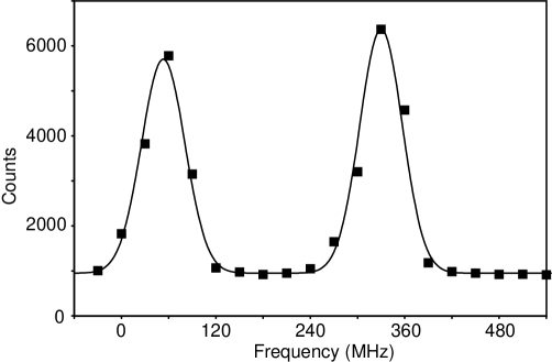
Figure 11: Scan with wavemeter reading. The dots are the number of photons per second and the solid line is a fit with two Gaussian functions plus a background. The origin is arbitrarily defined to be 13732.467 cm^-1 on the wavemeter. gomezF11.EPS.

The resolution of the wavemeter can be improved if one assumes that the noise is Gaussian. Fig. 11 shows a plot of the number of photons vs wavemeter reading. The origin is arbitrarily defined to be 13732.476 cm^-1 on the wavemeter. We fit the data with two Gaussian peaks plus a background. With this method we find a hyperfine separation of 277.3$\pm$5.4 MHz.

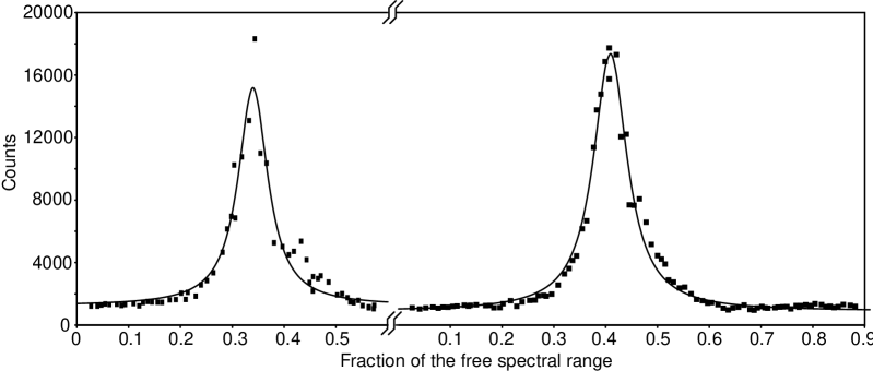
Figure 12: Scan with the cavity reading. The horizontal axis is the relative (or percent) position of the probe laser transmission peak with respect to two fixed He-Ne transmission peaks in the cavity. The dots are the number of photons per second and the solid line is a fit with a Lorentz function plus a background. The two peaks correspond to the two hyperfine levels and are separated by one free spectral range. gomezF12.EPS.

We perform several scans recording both the number of counts and the relative (or percent) position of the laser transmission peak with respect to two fixed He-Ne transmission peaks on the cavity. The result of a typical scan is shown in Fig. 12. The two peaks correspond to the two hyperfine levels and they are separated by one free spectral range. We fit each peak with a Lorentzian function plus a background and then average over all the scans. The difference in position between the two peaks is compared against the calibration to obtain the separation in MHz. The statistical uncertainty is the main contribution on the error budget (Table 3) with a 0.46$\%$ contribution.

The presence of a magnetic field may modify the hyperfine splitting measurement through a Zeeman splitting of the magnetic sublevels. Assuming all the atoms start from a common state and reach the highest magnetic sublevel on each of the hyperfine levels we obtain an upper limit for the contribution of the Zeeman shift of 0.16$\%$.

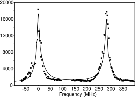
Figure 13: Solution of the steady state optical Bloch equations and its comparison with the data. The intensities and detunings of the beams were adjusted to approximate the data and are consistent with the experimental values. We also add a background and an overall scale to the simulation. The probe intensity used is 27 mW/cm², the repumper intensity is 37 mW/cm² and the repumper detuning is 3 MHz. gomezF13.EPS.

The presence of laser beams on the excitation can induce an AC shift and splitting of the hyperfine levels. We do not observe any clear asymmetry or splitting on each of the hyperfine peaks, although we do see some power broadening. The natural linewidth from the lifetime is 11.4 MHz, whereas the data has a linewidth of 24 MHz which shows power broadening. We model the scan signal by solving the steady state optical Bloch equationsgrossman00a and obtain an spectrum consistent with the data (Fig. 13). The intensities and detunings of the beams were adjusted to approximate the data and are consistent with the experimental ones. Using this model, we set limits for the effect of the AC Stark shift on the hyperfine splitting we measure to less than 0.2$\%$.

Table 3 summarizes the error budget for the measurement. We find a hyperfine splitting for the $7s$ level of 282.6$\pm$1.6 MHz.

The relation between the hyperfine shift and the magnetic dipole hyperfine constant (A) for an s level is given by

$$\frac{E_{HF}}{h}=A\frac{K}{2},$$ (13)

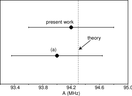
Figure 14: Result for the hyperfine constant measurement and comparison with: (a) previous experimental resultgupta73 and theoretical prediction safronova99 (dotted line). gomezF14.EPS.

with $K=F(F+1)-I(I+1)-J(J+1)$. In our case $I$=5/2 and $J$=1/2 so we have $A$=94.2$\pm$0.6 MHz. Fig. 14 shows a comparison of the present work with previous experimentsgupta73 and a theoretical prediction.safronova99 The theoretical prediction assumes a nuclear magnetic moment of 1.3534 in units of $\mu_{N}$ the nuclear magneton. We find good agreement between both experimental results and theory. Measurements of the hyperfine splitting of an $s$ level are useful to understand the contributions from radiative corrections such as the one produced by the Breit interaction.sushkov01

IV Conclusions

We have measured the lifetime and hyperfine splitting of the second excited $S_{1/2}$ level of Rb and the lifetime of the second excited $p$ manifold of Rb. We have used two-photon excitation and time-correlated single-photon counting techniques on a sample of cold ⁸⁵Rb atoms confined in a MOT. Our $7s$ lifetime measurement has excellent statistics and the result is limited by systematic uncertainties. The measurement represents a ten-fold improvement in the accuracy from previous measurements. The lifetime tests calculations of radial matrix elements connecting excited states in Rb. Comparisons with ab-initio calculations of the matrix elements for the different decay channels agree to better than 0.3%. The measurement of the lifetime of the $6p$ manifold does not differenciate between the two decay channels from the fine structure and achieves less accuracy, while a comparison to theory is model dependent, but sets bounds for the two contributions. The $0.57\%$ hyperfine splitting measurement is in agreement with previous values and theoretical calculations.

All these measurements confirm the high quality predictions of MBPT calculations and increase the confidence in the methods applied to heavier alkali atoms such as Fr and Cs for similar spectroscopic studies and extraction of weak interaction information from PNC measurements.

Table 1: Error budget for $7s$ level lifetime measurement.

Error	$[\%]$
Statistical	$\pm 0.17$
Trap displacement	$\pm 0.38$
Time calibration	$\pm 0.01$
TAC/MCA nonlinearity	$\pm 0.04$
Quantum beats	$<\pm 0.10$
Total	$\pm$0.43

Table 2: Error budget for $6p$ manifold lifetime measurement.

Error	$[\%]$
Statistical	$\pm 0.15$
$7s$ uncertainty propagation	$\pm 0.25$
Time calibration	$\pm 0.94$
Total	$\pm$0.98

Table 3: Error budget for $7s$ level hyperfine splitting measurement.

Error	$[\%]$
Statistical	$\pm 0.46$
Cavity calibration	$\pm 0.15$
Differential Zeeman shift	$\pm 0.16$
AC Stark asymmetrical broadening	$<\pm 0.20$
Total	$\pm$0.55

List of Figure Captions

Fig. 1. Energy levels of ⁸⁵Rb for trapping and two photon excitation to the $7s$ level (solid lines) fluorescence detection (dashed line) and undetected fluorescence (dotted line).

Fig. 2. Schematic of the trap. AM EOM stands for amplitude modulation with an electro-optic modulator and AM AOM for amplitude modulation with an acousto-optic modulator.

Fig. 3. Decay paths for the $7s$ and $6p$ levels of ⁸⁵Rb.

Fig. 4. Timing sequence for the excitation of atoms to the $7s$ level. High level is on, low level is off.

Fig. 5. Block diagram for the electronics used for the detection of $7s$ or $6p$ photons.

Fig. 6. Exponential decay of the $7s$ level. The upper plot contains the raw data that shows the excitation turn on and turn off as well as the exponential decay of the atoms (left scale). It also shows the background subtracted signal together with the exponential fit (right scale). The lower plot shows the normalized residuals (assuming statistical noise).

Fig. 7. Lifetime obtained when the trap is displaced by inserting a piece of glass in the retro-reflection mirrors of the MOT while the magnetic field environment remains unchanged. (a) no displacement, (b) displacement using mirror 1, (c) mirror 2, (d) mirror 3 and beams realigned, (e) no displacement and beams not realigned.

Fig. 8. Experimental result of the 7s lifetime in Rb, together with previous experimental results: (a)Marek et al,marek80 (b)Bulos et al,bulos76 and theoretical predictions: (c)Safronova et al,safronova03 (d)Theodosiou.theodosiou84

Fig. 9. Decay of the $6p$ manifold. The upper plot contains the raw data (left scale) and the data minus the background minus the exponential contribution from the $7s$ level (right scale). An exponential fit to this last curve is also shown. The lower plot contains the normalized residuals (assuming statistical noise).

Fig. 10. Constraints on the lifetimes of the two $6p$ fine levels in Rb using the model described in the text and the experimental result. The solid lines define the limits of the 1$\sigma$ and 2$\sigma$ regions respectively. The circles are theoretical predictions: (a)Safronova et al,safronova03 (b)Theodosiou.theodosiou84

Fig. 11. Scan with wavemeter reading. The dots are the number of photons per second and the solid line is a fit with two Gaussian functions plus a background. The origin is arbitrarily defined to be 13732.467 cm^-1 on the wavemeter.

Fig. 12. Scan with the cavity reading. The horizontal axis is the relative (or percent) position of the probe laser transmission peak with respect to two fixed He-Ne transmission peaks in the cavity. The dots are the number of photons per second and the solid line is a fit with a Lorentz function plus a background. The two peaks correspond to the two hyperfine levels and are separated by one free spectral range.

Fig. 13. Solution of the steady state optical Bloch equations and its comparison with the data. The intensities and detunings of the beams were adjusted to approximate the data and are consistent with the experimental values. We also add a background and an overall scale to the simulation. The probe intensity used is 27 mW/cm², the repumper intensity is 37 mW/cm² and the repumper detuning is 3 MHz.

Fig. 14. Result for the hyperfine constant measurement and comparison with: (a) previous experimental resultgupta73 and theoretical prediction safronova99 (dotted line).

Figure 1: Energy levels of ⁸⁵Rb for trapping and two photon excitation to the $7s$ level (solid lines) fluorescence detection (dashed line) and undetected fluorescence (dotted line). gomezF1.EPS.

References

- (1) W. R. Johnson, M. S. Safronova, and U. I. Safronova, “Combined effect of coherent Z exchange and the hyperfine interaction in the atomic parity-nonconserving interaction,” Phys. Rev. A 67, 062106-1 (2003).
- (2) J. S. M. Ginges, and V. V. Flambaum, “Violations of fundamental symmetries in atoms and tests of unification theories of elementary particles,” Phys. Rep. 397, 63-154 (2004).
- (3) C. S. Wood, S. C. Bennett, D. Cho, B. P. Masterson, J. L. Roberts, C. E. Tanner, and C. E. Wieman, “Measurement of parity nonconservation and an anapole moment in cesium,” Science 275, 1759-1763 (1997).
- (4) C. S. Wood, S. C. Bennett, J. L. Roberts, D. Cho, and C. E. Wieman, “Precision measurement of parity nonconservation in cesium,” Can. J. Phys. 77, 7-75 (1999).
- (5) S. K. Lamoreaux and I. B. Khriplovich, CP violation without strangeness (Springer Verlag, New York, 1997).
- (6) L. A. Orozco, “Precision tests of the Standard Model with trapped atoms,” in Trapped Particles and Fundamental Physics, Les Houches 2000, edited by S. N. Atutov, R. Calabrese, and L. Moi (Kluwer Academic Publishers, Amsterdam, 2002), pp. 125-159.
- (7) S. Aubin, E. Gomez, L. A. Orozco, and G. D. Sprouse, “High efficiency magneto-optical trap for unstable isotopes,” Rev. Sci. Instrum. 74, 4342-4351 (2003).
- (8) S. Aubin, E. Gomez, L. A. Orozco, and G. D. Sprouse, “Lifetime measurement of the level of atomic francium,” Opt. Lett. 28, 2055-2057 (2003).
- (9) S. Aubin, E. Gomez, L. A. Orozco, and G. D. Sprouse, “Lifetimes of the 9s and 8p levels of atomic francium,” submitted for publication.
- (10) R. D. Cowan, The theory of atomic structure and spectra (University of California Press, California, 1981).
- (11) W. Z. Zhao, J. E. Simsarian, L. A. Orozco, and G. D. Sprouse, “A computer-based digital feedback control of frequency drift of multiple lasers,” Rev. Sci. Instrum. 69, 3737-3740 (1998).
- (12) D. V. O’Connor and D. Phillips, Time Correlated Single Photon Counting (Academic, London, 1984).
- (13) L. Young, W. T. H. III, S. J. Sibener, S. D. Price, C. E. Tanner, C. E. Wieman, and S. R. Leone,“Precision lifetime measurements of Cs 6p2P1/2 And 6p2P3/2 levels by single-photon counting,” Phys. Rev. A 50, 2174-2181 (1994).
- (14) B. Hoeling, J. R. Yeh, T. Takekoshi, and R. J. Knize, “Measurement of the lifetime of the atomic cesium 52D5/2 state with diode-laser excitation,” Opt. Lett. 21, 74-76 (1996).
- (15) R. G. DeVoe and R. G. Brewer, “Precision-measurements of the lifetime of a single trapped ion with a nonlinear electrooptic switch,” Opt. Lett. 19, 1891-1893 (1994).
- (16) J. E. Simsarian, L. A. Orozco, G. D. Sprouse, and W. Z. Zhao, “Lifetime measurement of the 7 levels of francium,” Phys. Rev. A 57, 2448-2458 (1998).
- (17) J. M. Grossman, R. P. Fliller III, L. A. Orozco, M. R. Pearson, and G. D. Sprouse, “Lifetime measurements of the levels of atomic francium,” Phys. Rev. A 62, 062502 (2000).
- (18) M. S. Safronova, C. J. Williams, and C. W. Clark, “Relativistic many-body calculations of electric-dipole matrix elements, lifetimes and polarizabilities in rubidium,” Phys. Rev. A 69, 022509 (2004).
- (19) C. E. Theodosiou, “Lifetimes of alkali-metal atom Rydberg states,” Phys. Rev. A 30, 2881-2909 (1984).
- (20) J. Marek and P. Munster, “Radiative lifetimes of excited-states of rubidium up to quantum number n=12,” J. Phys. B 13, 1731-1741 (1980).
- (21) B. R. Bulos, R. Gupta, and W. Happer, “Lifetime measurements in excited s states of K, Rb, and Cs by cascade Hanle effect,” J. Opt. Soc. Am. 66, 426-433 (1976).
- (22) A. Derevianko, “Correlated many-body treatment of the Breit interaction with application to cesium atomic properties and parity violation,” Phys. Rev. A 65, 012106 (2001).
- (23) H. Kopfermann, Nuclear Moments (Academic Press, New York, 1958).
- (24) J. M. Grossman, R. P. Fliller III, Mehlstäubler, L. A. Orozco, M. R. Pearson, G. D. Sprouse, and W. Z. Zhao, “Energies and hyperfine splittings of the 7D levels of atomic francium,” Phys. Rev. A 62, 052507 (2000).
- (25) R. Gupta, W. Happer, L. K. Lam, and S. Svanberg, “Hyperfine-structure measurements of excited s states of the stable isotopes of potassium, rubidium, and cesium by cascade radio-frequency spectroscopy,” Phys. Rev. A 8, 2792-2810 (1973).
- (26) M. S. Safronova, W. R. Johnson, and A. Derevianko, “Relativistic many-body calculations of energy levels, hyperfine constants, electric-dipole matrix elements, and static polarizabilities for alkali-metal atoms,” Phys. Rev. A 60, 4476-4487 (1999).
- (27) O. P. Sushkov, “Breit-interaction correction to the hyperfine constant of an external s electron in a many-electron atom,” Phys. Rev. A 63, 042504 (2001).