Periodic orbits of the ensemble of Sinai-Arnold cat maps and pseudorandom number generation

Abstract

We propose methods for constructing high-quality pseudorandom number generators (RNGs) based on an ensemble of hyperbolic automorphisms of the unit two-dimensional torus (Sinai–Arnold map or cat map) while keeping a part of the information hidden. The single cat map provides the random properties expected from a good RNG and is hence an appropriate building block for an RNG, although unnecessary correlations are always present in practice. We show that introducing hidden variables and introducing rotation in the RNG output, accompanied with the proper initialization, dramatically suppress these correlations. We analyze the mechanisms of the single-cat-map correlations analytically and show how to diminish them. We generalize the Percival–Vivaldi theory in the case of the ensemble of maps, find the period of the proposed RNG analytically, and also analyze its properties. We present efficient practical realizations for the RNGs and check our predictions numerically. We also test our RNGs using the known stringent batteries of statistical tests and find that the statistical properties of our best generators are not worse than those of other best modern generators.

I Introduction

Molecular dynamics and Monte Carlo simulations are important computational techniques in many areas of science: in quantum physics Beach , statistical physics Landau2000 , nuclear physics Pieper , quantum chemistry Luechow , material science Bizzari , among many others. The simulations rely heavily on the use of random numbers, which are generated by deterministic recursive rules. Such rules produce pseudorandom numbers, and it is a great challenge to design random number generators (RNGs) that behave as realizations of independent uniformly distributed random variables and approximate “true randomness” Knuth .

There are several requirements for a good RNG and its implementation in a subroutine library. Among them are statistical robustness (uniform distribution of values at the output with no apparent correlations), unpredictability, long period, efficiency, theoretical support (precise prediction of the important properties), portability and others Knuth ; Lecuyer ; Brent .

A number of RNGs introduced in the last five decades fulfill most of the requirements and are successfully used in simulations. Nevertheless, each of them has some weak properties which may (or may not) influence the results.

The most widely used RNGs can be divided into two classes. The first class is represented by the Linear Congruential Generator (LCG), and the second, by Shift Register (SR) generator.

Linear Congruential Generators (LCGs) are the best-known and (still) most widely available RNGs in use today. An example of the realization of an LCG generator is the UNIX rand generator $y_{n}=(1103515245\;y_{n-1}+12345)\ (\bmod\ 2^{31})$. The practical recommendation is that LCGs should be avoided for applications dealing with the geometric behavior of random vectors in high dimensions because of the bad geometric structure of the vectors that they produce Knuth ; Coveyou .

Generalized Feedback Shift Register (GFSR) sequences are widely used in many areas of computational and simulational physics. These RNGs are quite fast and possess huge periods given a proper choice of the underlying primitive trinomials Golomb . This makes them particularly well suited for applications that require many pseudorandom numbers. But several flaws have been observed in the statistical properties of these generators, which can result in systematic errors in Monte Carlo simulations. Typical examples include the Wolff single cluster algorithm for the 2D Ising model simulation SR1 , random and self-avoiding walks Grass , and the 3D Blume–Capel model using local Metropolis updating SR3 .

Modern modifications and generalizations to the LCG and GFSR methods have much better periodic and statistical properties. Some examples are the Mersenne twister MT (this generator employs the modified and generalized GFSR scheme), combined LCGs generators CombinedLCG and combined Tausworthe generators CombinedTausw ; LFSR113 .

Most RNGs used today can be easily deciphered. Perhaps the generator with the best unpredictability properties known today is the BBS generator BBS ; BBSImpr , which is proved to be polynomial-time perfect under certain reasonable assumptions BBS ; Lecuyer if the size $s$ of the generator is sufficiently large. This generator is rather slow for practical use because its speed decreases rapidly as $s$ increases. The discussion of cryptographic RNG is beyond our analysis.

We propose using an ensemble of simple nonlinear dynamical systems to construct an RNG. Of course, not all dynamical systems are useful. For instance, baker’s transformation is a simple example of a chaotic system: it is area preserving and deterministic, and its state is maintained in a bounded domain. The base of baker’s transformation is the Bernoulli shift $x_{n+1}=2x_{n}\ (\bmod\ 1)$, it yields a sequence of random numbers provided we have a random irrational seed. But in real computation, the seed number has finite complexity, and the number of available bits decreases at each step. Obviously, there is no practical use of this scheme for an RNG.

The logistic map Licht ; Schuster also does not help to construct an RNG. First, manipulation with real values of fixed accuracy leads to significant errors during long orbits. Second, the sequence of numbers generated by a logistic map does not have a uniform distribution Schuster . Also, the logistic map represents a chaotic dynamical system only for isolated values of a parameter. Even small deviations from these isolated values lead to creating subregions in the phase space, i.e., the orbit of the point does not span the whole phase space.

The next class of dynamical systems is Anosov diffeomorphisms of the two-dimensional torus, which have attracted much attention in the context of ergodic theory. Anosov systems have the following stochastic properties: ergodicity, mixing, sensitive dependence on initial conditions (which follows from the positivity of the Lyapunov exponent), and local divergence of all trajectories (which follows from the positivity of the Kolmogorov–Sinai entropy). These properties resemble certain properties of randomness. Every Anosov diffeomorphism of the torus is topologically conjugate to a hyperbolic automorphism, which can be viewed as a completely chaotic Hamiltonian dynamical system. Hyperbolic automorphisms are represented by $2{\times}2$-matrixes with integer entries, a unit determinant, and real eigenvalues, and are known as cat maps (there are two reasons for this terminology: first, CAT is an acronym for Continuous Automorphism of the Torus; second, the chaotic behavior of these maps is traditionally described by showing the result of their action on the face of the cat ArnoldAvez ). We note that cat maps are Hamiltonian systems. Indeed, if $k=\mbox{Tr}(M)=m_{11}+m_{22}>2$, then the action of map (1) on the vector ${p\choose q}$ can be described as the motion in the phase space specified by the Hamiltonian Keating $H(p,q)=(k^{2}-4)^{-1/2}\sinh^{-1}((k^{2}-4)^{1/2}/2)(m_{12}p^{2}-m_{21}q^{2}+(m_{11}-m_{22})pq)$. Here, $p$ and $q$ are taken modulo $1$ at each observation (i.e., we preserve only the fractional part of $p$ and $q$; the integer part is ignored), and observations occur at integer points of time.

In this paper, we present RNGs based on an ensemble of cat maps and analyze the requirements for a good RNG with respect to our scheme. The basic idea is to apply the cat map to a discrete set of points (there are two modifications: for $g=2^{m}$ and for prime $g$, where $(g{\times}g)$ is the lattice) such that each point belongs to a different periodic trajectory.

A similar utilization of cat maps for an RNG is called the matrix generator for pseudorandom numbers. It was introduced in Grothe ; Niederr1 and discussed for prime values of $g$. But because the single matrix generator is a generalization of the linear congruential method, it suffers from both the defects of LCG AfferbachGrothe and the defects of GFSR (see Sec. IV). The periodic and statistical properties of the matrix generators and of the equivalent multiple recursive generators have been studied NeiderrSerial ; Lecuyer98 , but the single $2{\times}2$-matrix generator still has significant correlations between values at the output.

Also, there is an impressive theoretical basis for relating properties of the periodic orbits of cat maps and properties of algebraic numbers PercivalVivaldi , which to the best of our knowledge has never been directly applied to RNG theory. Applying the ensemble of matrix transformations of the two-dimensional torus while using only a single bit from the point of each map, and utilizing rotation in the RNG output are the distinctive features of our generator. Also, as for other generators, a proper initialization of the initial state is important. As will be seen, the proposed scheme has several advantages. First, it can essentially reduce correlations and lead to creating an RNG not worse than other modern RNGs. Second, both the properties of periodic orbits and the statistical properties of such a generator can be analyzed both theoretically and empirically. Several examples of RNGs made by this method, as well as the effective realizations, are presented.

The generator is introduced in Sec. II. In Sec. III, we present the results for stringent statistical tests. Correlations for a single cat map are also analyzed thoroughly, and some correlations are found by the random walks test. We analyze the mechanism of these correlations in Sec. IV; they appear to be associated with the geometric properties of the cat map. We find these correlations analytically (Sec. IV). We provide a method for obtaining quantities such as the periods of cat maps, the number of orbits with a given period, and the area in the phase space swept by the orbits with a given period (Appendix A). We also provide a method for obtaining periods of the generator for arbitrary parameters of the map and lattice (Appendix B). This gives the primary theoretical support of the generator. In particular, we find that the typical period of the generator for the $2^{m}{\times}2^{m}$ lattice is $T_{m}=3\cdot 2^{m-2}$. The method is based on the work of Percival and Vivaldi, who transformed the study of the periodic orbits of cat maps into the modular arithmetic in domains of quadratic integers. The key ideas needed for our consideration are briefly reviewed in Appendix A. Appendix C gives the method for analyzing correlations between orbits of different points and choosing the proper initial conditions to minimize the correlations. Appendix D and supplemental details SpaceProofCite support the other sections, giving detailed proofs of the underlying results. Appendix E presents the efficient realizations for several versions of RNG, the initialization techniques, and the analysis of the speed of the RNGs.

II The Generator

II.1 Description of the method

We consider hyperbolic automorphisms of the unit two-dimensional torus (the square $(0,1]\times(0,1]$ with the opposite sides identified). The action of a given cat map $R$ is defined as follows: first, we transform the phase space by the matrix

$$M=\left(\begin{array}[]{cc}m_{11}&m_{12}\\ m_{21}&m_{22}\\ \end{array}\right)\in SL_{2}({\mbox{\myBbb Z}});$$ (1)

second, we take the fractional parts in $(0,1)$ of both coordinates. Here $SL_{2}({\mbox{\myBbb Z}})$ denotes the special linear group of degree $2$ over the ring of integers, i.e., the elements of $M$ are integers, $\det M=1$, and the eigenvalues of $M$ are $\lambda=(k\pm\sqrt{k^{2}-4})/2$, where $k={\rm Tr}(M)$ is the trace of the matrix $M$. The eigenvalues should be real because complex values of $\lambda$ lead to a nonergodic dynamical process, and the hyperbolicity condition is $|k|>2$.

It is easy to prove that the periodic orbits of the hyperbolic toral automorphism $R$ consist precisely of those points that have rational coordinates ArnoldAvez ; PercivalVivaldi ; Keating . Hence, it is natural to consider the dynamics of the map defined on the set of points with rational coordinates that share a given denominator $g$. The lattice of such points is invariant under the action of the cat maps. In practice, we construct generators with $g=2^{m}$, where $m$ is a positive integer, and generators with $g=p=2^{m}-1$, where $m$ is a Mersenne exponent, i.e., $p=2^{m}-1$ is a prime.

The notion of an RNG can be formalized as follows: a generator is a structure ${\cal G}=(S,s_{0},T,U,G)$, where $S$ is a finite set of states, $s_{0}\in S$ is the initial state (or seed), the map $T:S\rightarrow S$ is the transition function, $U$ is a finite set of output symbols, and $G:S\rightarrow U$ is the output function Lecuyer . Thus, the state of the generator is initially $s_{0}$, and the generator changes its state at each step, calculating $s_{n}=T(s_{n-1})$, $u_{n}=G(s_{n})$ at step $n$. The values $u_{n}$ at the output of the generator are called the observations or the random numbers produced by the generator. The output function $G$ may use only a small part of the state information to calculate the random number, the majority of the information being ignored. In this case, there exist hidden variables, i.e., some part of the state information is “hidden” and cannot be restored using only the sequence of RNG observations.

We consider the generator with $S=L^{s}$, where $L=\{0,1,\dots,g-1\}\times\{0,1,\dots,g-1\}$ is the lattice on the torus and $s$ is a positive integer. In other words, the state consists of coordinates of $s$ points of the $g{\times}g$ lattice on the torus. For instance, the initial state consists of points ${x_{i}^{(0)}\choose y_{i}^{(0)}}$, where $x_{i}^{(0)},y_{i}^{(0)}\in\{0,1,\dots,g-1\}$ and $i=0,1,\dots,(s-1)$. We note that these are points of the integer lattice, i.e., $x_{i}^{(0)}$ and $y_{i}^{(0)}$ are positive integers. The actual initial points on the unit two-dimensional torus $(0,1]\times(0,1]$ are

$${x_{i}^{(0)}/g\choose y_{i}^{(0)}/g},\quad i=0,1,\dots,(s-1).$$ (2)

The transition function of the generator is defined by the action of the cat map $R$, i.e., these $s$ points are affected at every step by the cat map:

$${x_{i}^{(n)}/g\choose y_{i}^{(n)}/g}=M{x_{i}^{(n-1)}/g\choose y_{i}^{(n-1)}/g}\ (\bmod\ 1),\quad i=0,1,\dots,(s-1).$$ (3)

Here the $\bmod\ 1$ operation means taking the fractional part in $(0,1)$ of the real number. An equivalent description of the transition function is

$${x_{i}^{(n)}\choose y_{i}^{(n)}}=M{x_{i}^{(n-1)}\choose y_{i}^{(n-1)}}\ (\bmod\ g),\quad i=0,1,\dots,(s-1).$$ (4)

We let $\alpha_{i}^{(n)}$ denote $0$ or $1$ depending on whether $x_{i}^{(n)}<(g/2)$ or $x_{i}^{(n)}\geq(g/2)$, i.e., $\alpha_{i}^{(n)}=\lfloor 2x_{i}^{(n)}/g\rfloor$. The output function of the generator $G:L^{s}\rightarrow\{0,1,\dots,2^{s}-1\}$ is defined as $a^{(n)}=\sum_{i=0}^{s-1}\alpha_{i}^{(n)}\cdot 2^{i}$. In other words, $a^{(n)}$ is an $s$-bit integer consisting of the bits $\alpha_{0}^{(n)},\alpha_{1}^{(n)},\dots,\alpha_{s-1}^{(n)}$. In the case $g=2^{m}$, $a^{(n)}$ contains precisely the first bits of the integers $x_{0}^{(n)},x_{1}^{(n)},\dots,x_{s-1}^{(n)}$. The sequence of random numbers produced by the generator is $\{a^{(n)}\}$.

We see that the constructed RNG has much hidden information. For example, if $g=2^{m}$, then $s(m{-}1)$ bits of ${x_{i}^{(n)}\choose y_{i}^{(n)}}$ are the hidden variables; these are the bits that are not involved in constructing the value of the output function $a^{(n)}$.

Thus, applying the chaotic behavior of Anosov motion and introducing an ensemble of systems while keeping part of the information hidden are the main ingredients of the proposed method. Good stochastic properties of the underlying continuous system are obviously necessary for good generators. For example, the logarithm of the multiplier in the continuous transformation of the LCG can be viewed as the Lyapunov exponent, which is always greater than $1$, and this leads to the divergence of trajectories. The huge number of points on a lattice makes the continuous system a good first approximation to the RNG and leads to the importance of good chaotic properties. Introducing hidden variables reduces correlations (as is shown in Sec. III).

The calculation of the period of the RNG is presented in Appendix B. The typical period length is $T_{m}=3\cdot 2^{m-2}$ for the $2^{m}{\times}2^{m}$ lattice. The proper initializations for the generators are presented in Appendix E. The proper initialization guarantees that the actual period is not smaller than $T_{m}$ and that the points ${x_{i}^{(0)}\choose y_{i}^{(0)}}$, $i=0,1,\dots,(s-1),$ belong to different orbits of the cat map.

II.2 Connection with other generators

There are several known connections between Anosov dynamical systems and pseudorandom number generation.

First, the concept of the Shift Register Sequence, which is widely used to construct high-quality RNGs, is connected to dynamical systems (see, e.g., the discussion in SB-dyn ). Let the state of the shift register be ${\bf v_{n-1}}=(a_{n-r},a_{n-r+1},\dots,a_{n-1})$. At the next iteration, the state of the shift register is ${\bf v_{n}}=(a_{n-r+1},a_{n-r+2},\dots,a_{n})$, where $a_{n}=c_{r}a_{n-r}+c_{s}a_{n-s}\ (\bmod\ 2)$. In other words, ${\bf v_{n+1}}=A{\bf v_{n}}\ (\bmod\ 2)$, where $A$ is an $(r{\times}r)$-matrix.

Second, LCGs in some cases can be described by the action of the hyperbolic toral automorphism Bonelli .

Last, it can be shown that, for each $i$, the sequence $\{x_{i}^{(n)}\}$, defined above, as well as the sequence $\{y_{i}^{(n)}\}$, follows a linear recurrence modulo $g$:

$$x^{(n)}=kx^{(n-1)}-qx^{(n-2)}\ (\bmod\ g)$$ (5)

$$y^{(n)}=ky^{(n-1)}-qy^{(n-2)}\ (\bmod\ g),$$ (6)

where $k=\mbox{Tr}(M)$, and $q=\det M=1$. The characteristic polynomial of the last linear recurrence is $f(x)=q-kx+x^{2}$, which is exactly the same as that of the matrix $M$ Grothe ; Lecuyer90 .

The period properties of sequence (5) follow from the arithmetical methods for $q=1$ (see Appendix A and Appendix B) and from the finite field theory in the case where $g=p$ is a prime Knuth .

II.3 Generators for prime $g$: modifications for $\det M=1$ and for $\det M\neq 1$

The matrix generator of pseudorandom numbers equivalent to sequence (5) was studied in Knuth ; Grothe ; NiederrBook in the case where $g=\det M=p$ is a prime. Sequence (5) yields the maximum possible period $p^{2}{-}1$ if and only if the characteristic polynomial $f(x)$ is primitive over ${\mbox{\myBbb Z}}_{p}$. But for $q=1$ the polynomial $f(x)=x^{2}-kx+1$ is not primitive over ${\mbox{\myBbb Z}}_{p}$ for $p>2$. Therefore, if $\det M=1$, the period is always smaller than $p^{2}-1$. An even stronger result follows from PercivalVivaldi : the period cannot be larger than $p+1$ when $g$ is a prime and $\det M=1$.

Matrix generators with $q\neq 1$ are not immediately connected with Hamiltonian dynamical systems. Indeed, the transformation with $\det M\neq 1$ does not preserve the volume in phase space and does not immediately represent a cat map. However, whatever $q$ is, we have $\det M^{p-1}\equiv 1\ (\bmod\ p)$. This means that the action of the matrix $M^{p-1}$ on a lattice $p\times p$ is exactly the same as the action of a unimodular matrix. Therefore, any orbit of a “non-Hamiltonian” transformation $M$ contains exactly $p-1$ cat-map orbits.

Also, transformations with $q=1$ preserve the norm on the orbit modulo $g$ (see Appendix C), in contrast to transformations with $q\neq 1$. It is shown in Appendix C that some of the correlations between the orbits are inherent in the case $q=1$ and are suppressed for $q\neq 1$.

II.4 Rotating the RNG output

It will be seen that in the scheme of the generator, there are correlations between the first bits of $a^{(n)}$, correlations between the second bits of $a^{(n)}$, and so on. To suppress these correlations, we modify the algorithm as follows. At each step, we renumber the points in the generator output: $1\rightarrow 2,2\rightarrow 3,\dots,s\rightarrow 1$. In other words, the bits inside $a^{(n)}$ are rotated, and the RNG output function is defined as $b^{(n)}=\sum_{i=0}^{s-1}\alpha_{i}^{(n)}\cdot 2^{(i+n)\ (\bmod\ s)}$ instead of $a^{(n)}=\sum_{i=0}^{s-1}\alpha_{i}^{(n)}\cdot 2^{i}$, where $\alpha_{i}^{(n)}=\lfloor 2x_{i}^{(n)}/g\rfloor$.

The main advantage of the modified algorithm is that it leads to decreasing the correlations of the values $a^{(n)}$ between each other. For example, we will see in Sec. IV that the rotation strongly reduces the specific correlations found by the random walks test.

We note that the rotating the bits in the RNG output does not deteriorate any properties of the RNG provided that $s$ divides the period of free orbits $T_{m}$ (in practice, this is a very realistic condition). In particular, neither does the generator period become smaller (see Appendix B), nor do the statistical properties become worse.

Rotating the bits in the RNG output is thus a practically useful modification. In addition, the rotation makes deciphering an even more complicated problem.

III Statistical tests

III.1 Simple Knuth tests

In this section, we present the results of several standard statistical tests Knuth that reveal the correlation properties of the generator described in Sec. II. Namely, the frequency test, serial test, maximum-of-t test, test for monotonic subsequences (“run test”) and collision test were applied for an RNG with $M={2\ 3\choose 3\ 5}$, $g=2^{m}=2^{28}$ and $s=28$ points in the state. All the statistical tests were passed. All empirical tests except the collision test (CT) are based on either the chi-square test ($\chi^{2}$) or the Kolmogorov–Smirnov test (KS). We follow Knuth’s notation Knuth .

The results of the tests are presented in Table 1, where $n$ is the number of values of $a^{(n)}$ for each test (for the serial test, $n$ is the number of pairs $\{a^{(2n)},a^{(2n+1)}\}$) and $\nu$ is the number of degrees of freedom. For the serial test $d=8$, i.e., we used exactly $3$ bits of each $a^{(n)}$ number; hence, $\nu=d^{2}-1=63$. For the run test, $\nu=5$ means that we sought monotonic subsequences of lengths 1,2,3,4,5 and of length $\geq 6$.

For all of the KS tests, the empirical distributions of $P(K^{+})$ and $P(K^{-})$ were calculated, where $P(x)$ is the theoretical Kolmogorov–Smirnov distribution Knuth . Figure 1 shows these empirical distributions for the frequency test. These distributions lead to their own values of $K^{+}$ and $K^{-}$: the values $P(K^{\prime+})$ and $P(K^{\prime-})$ characterizing the empirical distribution of $K^{+}$ and the values $P(K^{\prime+})$ and $P(K^{\prime-})$ characterizing the empirical distribution of $K^{-}$. These values are presented in Table 1. Our RNG passes all the KS tests because the values $K^{+}$ and $K^{-}$ are distributed in accordance with the theory prediction. For each chi-square test, the empirical distribution of 20 values of $P(V)$ was calculated. In our tests, it looks similar to those shown in Fig. 1, where $P(x)$ is the theoretical chi-square distribution and $V$ is the output of the chi-square test. For each collision test, the number of collisions $c$ and the theoretical probability $P(c)$ that the number of collisions is not larger than $c$ were calculated. The empirical distribution of $P(c)$ was analyzed, and the results are also presented in Table 1.

Table 1: Results of the statistical tests for the RNG based on the ensemble of cat maps (see Sec. II) with parameters $M={2\ 3\choose 3\ 5}$, $g=2^{m}=2^{28}$, $s=28$.

Test	Parameters	Number and		Tests output values	Distribution of $V_{1}$		Distribution of $V_{2}$		Conclusion
		type of tests		$V_{1}$ and $V_{2}$	$P(K^{\prime+})$	$P(K^{\prime-})$	$P(K^{\prime+})$	$P(K^{\prime-})$
Frequency test	$n=10^{6}$	$20$	KS	$V_{1}=K^{+},V_{2}=K^{-}$	$0.592392$	$0.174451$	$0.457758$	$0.473379$	PASSED
Serial test	$n=10^{6},d=8$	$20$	$\chi^{2}$	$V_{1}=V$	$0.837112$	$0.17128$	n/a	n/a	PASSED
Run test	$n=10^{6},\nu=5$	$20$	$\chi^{2}$	$V_{1}=V$	$0.383601$	$0.805434$	n/a	n/a	PASSED
Maximum-of-t test	$n=10^{6},t=5$	$20$	KS	$V_{1}=K^{+},V_{2}=K^{-}$	$0.120912$	$0.765201$	$0.704026$	$0.589702$	PASSED
Collision test	$m=2^{20},n=2^{14}$	$20$	CT	$V_{1}=c$	$0.150537$	$0.858955$	n/a	n/a	PASSED

Figure 1: Distribution of $P(K^{+})$ and $P(K^{-})$ for the frequency test. The test was performed for the RNG from Sec. II with the parameters $M={2\ 3\choose 3\ 5}$, $g=2^{m}=2^{28}$, $s=28$.

We note that all the empirical tests here except the collision test are essentially multibit. This means that the whole ensemble of cat maps influences the test result, and one can guess that hidden variables inside the generator is one reason for the successful test results. A single-bit cat-map generator, i.e., a generator from Sec. II with $s=1$, does not contain hidden variables. Most of the tests for a single-bit cat-map generator are also successfully passed. Namely, the frequency test and the serial test, which were modified for a one-bit generator, and the collision test are passed. But there are correlations in the single-bit cat-map generator (discussed later in this paper), and the most convenient method for observing them is the random walks test with $\mu=1/2$ (see Sec. IV). The random walks test is not the only test that can reveal the single-bit cat-map correlations. The same correlations are also observed by improved versions of some of the standard tests, e.g., the serial test for subsequences of length 5. Of course, many tests in Sec. III.2 would not be passed by a single-bit cat-map generator.

For comparison, we analyzed a simple generator based on the single cat map. Table 2 shows that such a generator with the transition function defined as ${x^{(n)}\choose y^{(n)}}=M{x^{(n-1)}\choose y^{(n-1)}}\ (\bmod\ 1)$ and the output function defined as $u_{n}=x^{(n)}$ has very bad properties. Of course, the frequency test is passed, since the trajectories of a cat map uniformly fill the phase space. But all the other tests are failed. Therefore, the simple generator based on the single cat map does have strong correlations in the output and is not useful practically.

Table 2: Results of the statistical tests for a simple RNG based on the single cat map with parameters $M={2\ 3\choose 3\ 5}$, $g=2^{m}=2^{28}$.

Test	Parameters	Number and		Tests output	Distribution of $V_{1}$		Distribution of $V_{2}$		Conclusion
		type of tests		values $V_{1}$, $V_{2}$	$P(K^{\prime+})$	$P(K^{\prime-})$	$P(K^{\prime+})$	$P(K^{\prime-})$
Frequency test	$n=10^{7}$	$20$	KS	$K^{+};K^{-}$	$0.96235$	$0.170581$	$0.787296$	$0.067341$	PASSED
Serial test	$n=5\cdot 10^{6},d=8$	$20$	$\chi^{2}$	$V$	$0.989499$	$0.006013$	n/a	n/a	FAILED
Run test	$n=10^{6},\nu=5$	$20$	$\chi^{2}$	$V$	$0$	$1$	n/a	n/a	FAILED
Maximum-of-t test	$n=10^{6},t=5$	$20$	KS	$K^{+};K^{-}$	$0$	$1$	$0$	$1$	FAILED
Collision test	$d=4,m=2^{10},n=2^{14}$	$20$	CT	$c$	$0$	$1$	n/a	n/a	FAILED

III.2 Batteries of stringent statistical tests

Knuth tests are very important but still not sufficient for the present-day sound analysis of the RNG statistical properties. Hundreds of statistical tests and algorithms are available in software packages, for example, widely used packages DieHard Diehard , NIST NIST and TestU01 TestU01 . All of them include tests, described by Knuth Knuth , as well as many other tests.

Table 3 shows the summary results for the SmallCrush, PseudoDiehard, Crush and Bigcrush batteries of tests from TestU01 . SmallCrush, PseudoDiehard, Crush and Bigcrush contain 14, 126, 93 and 65 tests respectively. The detailed parameters and initializations for the generators GS, GR, GSI, GRI, GM19 and GM31, based on the scheme proposed in Sec. II, are given in Appendix E.

For comparison, we also test several other generators, namely, the standard generators RAND, RAND48 and RANDOM and the modern generators MT19937, MRG32k3a and LFSR113. RAND is the simple LCG generator based on the recursion $x_{n}=(1103515245\;x_{n-1}+12345)\ (\bmod\ 2^{31})$. RAND48 is the 64-bit LCG based on the recursion $x_{n}=25214903917\;x_{n-1}+11\ (\bmod\ 2^{48})$. RANDOM provides an interface to a set of five additive feedback random number generators. RAND, RAND48 and RANDOM are implemented in the functions rand(), rand48() and random() in the standard Unix or Linux C library stdlib (see the documentation to rand(), rand48() and random()). MT19937 is the 2002 version of the Mersenne Twister generator of Matsumoto and Nishimura MT , which is based on the recent generalizations to the GFSR method. MRG32k3a is the combined multiply recursive generator proposed in CombinedLCG , and LFSR113 is a combined Tausworthe generator of L’Ecuyer LFSR113 .

The detailed statistics for the batteries of tests and the explicit results for every single test from the batteries can be found in AlgSite .

Table 3: Numbers of failed tests for the batteries of tests SmallCrush, Crush, Bigcrush TestU01 , and DieHard Diehard . Here $k=\mbox{Tr}(M)$ and $q=\det M$ are the RNG parameters (see Sec. II and Appendix E). For each test, we present three numbers: the number of statistical tests with p-values outside the interval $[10^{-2},1-10^{-2}]$, number of tests with p-values outside the interval $[10^{-5},1-10^{-5}]$, and number of tests with p-values outside the interval $[10^{-10},1-10^{-10}]$.

Generator	$k$	$q$	SmallCrush	Diehard	Crush	Bigcrush
GS	$3$	$1$	$0,0,0$	$44,29,29$	$20,16,14$	$22,20,19$
GR	$3$	$1$	$0,0,0$	$5,0,0$	$5,1,0$	$15,10,7$
GSI	$11$	$1$	$0,0,0$	$1,0,0$	$10,1,0$	$13,7,6$
GRI	$11$	$1$	$1,0,0$	$6,0,0$	$5,0,0$	$13,6,5$
GM19	$15$	$28$	$0,0,0$	$2,0,0$	$2,0,0$	$3,0,0$
GM31	$7$	$11$	$0,0,0$	$2,0,0$	$3,0,0$	$1,0,0$
RAND	$-$	$-$	$13,13,12$	$88,84,82$	$102,100,100$	$85,83,79$
RAND48	$-$	$-$	$5,5,3$	$27,23,22$	$22,20,20$	$27,23,22$
RANDOM	$-$	$-$	$3,2,2$	$17,15,15$	$13,11,10$	$21,15,14$
MRG32k3a	$-$	$-$	$1,0,0$	$3,0,0$	$4,0,0$	$2,0,0$
LFSR113	$-$	$-$	$0,0,0$	$3,0,0$	$8,6,6$	$8,3,3$
MT19937	$-$	$-$	$0,0,0$	$2,0,0$	$1,0,0$	$4,0,0$

We consider the test “failed” if the p-value lies outside the region $[10^{-2},1-10^{-2}]$. Most of the p-values for the failed tests for the cat-map generators are of the order of $10^{-3}$ to $10^{-5}$, but several are very small. We believe that the reason for small p-values is connected with the small period of the generators GS, GR, GSI, GRI and UNIX RAND. A period of the order of $3\cdot 10^{9}$, while sufficient for some applications, is not sufficient for many of the tests from Crush and Bigcrush. Therefore, the generators GS, GR, GSI and GRI demonstrate smaller p-values and larger numbers of failed tests from Crush and Bigcrush.

The existence of linear congruential dependences between orbits is another reason for small p-values for GS, GR, GSI and GRI. These correlations are described analytically in Appendix C. The GM19 and GM31 generators, having a period sufficient for the Crush and Bigcrush batteries, are simultaneously free from the linear congruential dependences. Therefore, they demonstrate much better statistical properties in Table 3.

Because we apply hundreds of tests, the number of failed tests is susceptible to random statistical flukes, especially when the p-values of failed tests lie in the suspect region $[10^{-2},10^{-5}]\cup[1-10^{-2},1-10^{-5}]$. Table 4 illustrates the flukes by showing the results of all batteries of tests for the generator GM31. The batteries were executed in the order SmallCrush, SmallCrush, PseudoDiehard, PseudoDiehard, Crush, Crush, BigCrush and BigCrush, i.e. each battery was executed twice. For the tests in Tables 3 and 4, the generator GM31 was initialized with identical parameters, in accordance with Appendix E. The numbers of failed tests themselves in Table 3 and Table 4 approximately indicate the statistical robustness of the generators. But if the p-value lies in the suspect region, one does not know exactly whether systematic correlations were found in the RNG or a statistical fluke occured.

Table 4: Applying each battery of tests twice for the GM31 generator. Here the test is considered failed if the p-value lies outside the interval $[10^{-2},1-10^{-2}]$

. Number of Failed tests, testing first time Failed tests, testing second time failed Tests No Name p-value No Name p-value SmallCrush 0/0 $-$ $-$ $-$ $-$ $-$ $-$ PseudoDiehard 3/2 1 BirthdaySpacings $0.0071$ 6 CollisionOver $0.0014$ 6 CollisionOver $0.999$ 7 CollisionOver $0.0018$ 14 Run of U01 $0.0093$ Crush 2/2 70 Fourier1, $r=0$ $0.0095$ 14 BirthdaySpacings, $t=7$ $0.0024$ 71 Fourier1, $r=20$ $0.0093$ 70 Fourier1, $r=0$ $0.0033$ BigCrush 4/3 6 MultinomialBitsOver $0.0014$ 32 SumCollector $0.0067$ 23 Gap, $r=0$ $0.9970$ 36 RandomWalk1 J(L=90) $0.9952$ 27 CollisionPermut $0.0052$ 41 RandomWalk1 J(L=10000) $0.9965$ 39 RandomWalk1 H(L=1000) $0.9982$

We conclude that the best of the generators based on cat maps are competitive with other good modern generators. In particular, we recommend the RNG realizations for GRI and GM31 for practical use. In Appendix E, we present the effective realizations of the generators GRI-SSE and GM31-SSE and recipes for the proper initialization. Among the generators examined here these are the best respective realizations with $g=2^{m}$ and with prime $g$.

IV The Random Walks Test

Analyzing the statistical properties of the generator theoretically is another important challenge. Such an analysis is traditionally performed by discussing the lattice structure Lecuyer98 ; Lecuyer90 ; AfferbachGrothe and discussing the discrepancy NiederrRev . The discrepancy of a matrix generator was analyzed by Niederreiter NeiderrSerial , who in particular, proved that the behavior of the discrepancy is strongly connected to the behavior of an integer called the figure of merit. Although calculating the exact values of the figure of merit would give an excellent basis for the practical selection of matrices for matrix generators, these values are still very hard to compute. To the best of our knowledge, this calculation has never been done for matrix generators of pseudorandom numbers.

Because of the hidden variables, the lattice structure of the matrix generator does not directly influence the statistical properties of the RNG introduced in Sec. II. Instead, we seek other kinds of correlations using the random walks test. The random walks test proved sensitive and powerful for revealing correlations in RNGs. In particular, correlations in the shift register RNG were found SR2 and explained SB ; RandomWalksTest using the random walks tests. In addition, the random walks test is a useful tool for analysis: if it fails, it gives the opportunity to understand the nature of the correlations for a particular RNG S99 .

There are several variations of the random walks test in different dimensions MonteCarloBook . We consider the one-dimensional directed random walk model RandomWalksTest : a walker starts at some site of an one-dimensional lattice, and at discrete times $i$, he either takes a step in a fixed direction with probability $\mu$ or stops with probability $1-\mu$. In the latter case, a new walk begins. The probability of a walk of length $n$ is $P(n)=\mu^{n-1}(1-\mu)$, and the mean walk length is $\langle n\rangle=1/(1-\mu)$. We note that the Ising simulations using cluster updates with the Wolff method are closely related to the random walk problem SB . Namely, the mean cluster size in the Wolff method equals the mean walk length for $\mu=\tanh(J/k_{B}T)$, where $J$ is the strength of the spin coupling and $T$ is the temperature.

Figure 2 shows the correlations in the RNG found by the random walks test. We applied 100 chi-square tests. Each test performed $n=10^{7}$ random walks with $\mu=1/2$ for a generator with $M={2\ 3\choose 3\ 5}$, $m=32$ and $s=1$. The result of the test with $\mu=1/2$ is independent of $s$ because only the first bit of the RNG is taken into account. For each test, the value $\delta P_{l}=(Y_{l}-np_{l})/(np_{l})$ was calculated for all walk lengths $l\leq 7$. Here $p_{l}$ is the theoretical probability of the walk length $l$ for uncorrelated random numbers, and $Y_{l}$ is the simulated number of walks with length $l$. We note that correlations can be found only for a large number of random walks (see Table 6), and no correlations are found even for $n=6\cdot 10^{4}$ random walks.

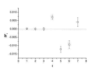
Figure 2: The deviation $\delta P_{l}$ of the probability of a walk length $l$ from the value for uncorrelated random numbers versus walk length $l$. The mean and the variance for $\delta P_{l}$ are represented for 100 chi-square random walk simulations. See the text for the details.

These correlations can be explained as follows. There are 32 five-bit sequences, and they do not have the same frequency of appearing in the RNG output. We consider one of them, for example, 10011. Let $X=(0,\frac{1}{2}]\times(0,1]$ and $Y=(\frac{1}{2},1]\times(0,1]$, i.e., $X$ and $Y$ are the left and the right halves of the torus. Let $x$ be the initial point $x_{0}^{(0)}\choose y_{0}^{(0)}$ of the generator. For the first bits of the first five outputs of the generator to be 10011, it is necessary and sufficient to have $x\in Z_{10011}=Y\cap R^{-1}(X)\cap R^{-2}(X)\cap R^{-3}(Y)\cap R^{-4}(Y)$. Here, $R$ is the action of the cat map. The set $Z_{10011}$ consists of filled polygons. Each polygon can be calculated exactly. The area $S(Z_{10011})$ equals the probability for the first five outputs of the generator to be 10011. This shows that the nature of the correlations is found in the geometric properties of the cat map.

Figure 3 (the left picture) represents the polygons corresponding to the subsequences of length three for the cat map with $M={2\ 3\choose 3\ 5}$. Each set of polygons, e.g., $Z_{010}=X\cap R^{-1}(Y)\cap R^{-2}(X)$, represents the region on the torus for the first initial point of the RNG and is drawn with its own color. The right picture represents the subsequences of length five for the cat map with $M={1\ 1\choose 1\ 2}$. Here, each set of polygons represents the regions on the torus for the third point of the generator, e.g., $\tilde{Z}_{01001}=R^{-2}(X)\cap R^{-1}(Y)\cap X\cap R(X)\cap R^{2}(Y)$, and is drawn with its own color. Of course, $S(\tilde{Z}_{01001})=S(Z_{01001})=P(01001)$ because the cat maps are area preserving. Therefore, the choice of pictures of $Z_{i}$ or pictures of $\tilde{Z}_{i}$ is unimportant if we only want to calculate the areas. Thus, the geometric structures in Fig. 3 show the regions of $Z_{000},\dots,Z_{111}$ (the left picture) or $\tilde{Z}_{00000},\dots,\tilde{Z}_{11111}$ (the right picture) and illustrate the geometric approach to calculating the probabilities.

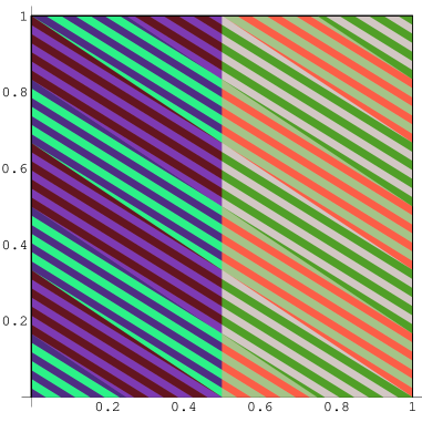
Figure 3: (Color online) Left: the regions on the torus for the first initial point of the RNG described in Sec. II with $M={2\ 3\choose 3\ 5}$. These regions correspond to the sequences $000,001,010,011,100,101,110$ and $111$ of the first bits generated by the RNG. Each region is drawn with its own color. Right: the regions on the torus for the third point of the RNG described in Sec. II with $M={1\ 1\choose 1\ 2}$. These regions correspond to the sequences of length 5 of the first bits generated by the RNG. Each region is drawn with its own color.

The exact areas $S(Z_{00000}),\dots,S(Z_{11111})$ can be easily calculated for various toral automorphisms. We prove the following geometric propositions:

1. In any case, every subsequence of length $3$, $2$ or $1$ respectively has the same probability $1/8$, $1/4$ or $1/2$.

2. If $k={\rm Tr}(M)$ is an odd number, then every subsequence of length $4$ has the same probability $P_{0}=1/16$.

3. If $k$ is even, then the probability of the subsequence $0000$ depends only on the trace $k$ of matrix $M$ of the cat map. It equals $P=P_{0}\cdot k^{2}/(k^{2}-1)$, where $P_{0}=1/16$.

The line of reasoning is presented in SpaceProofCite . Of course, the probability of the subsequence $0000$ automatically gives the probabilities of all other subsequences of length 4. We note that if $k$ is odd, then ideal $\langle 2\rangle$ is inert (see Appendix A.3), and the inert case is the easiest for exact analysis of the RNG period (see Appendices A and B). The probabilities of the subsequences of length 5 for maps with odd traces and of the subsequences of length 4 for maps with even traces are calculated exactly and shown in Table 5. It can be conjectured from Table 5 that if $k$ is odd, then the probability of the subsequence $00000$ of length 5 equals $P_{0}\cdot(1+1/(3k^{2}-6))$, where $P_{0}=1/32$.

Table 5: The probabilities of subsequences for different cat maps, characterized by the trace $k$.

$k$	$P(0000)/P_{0}$	$k$	$P(0000)/P_{0}$	$k$	$P(00000)/P_{0}$
4	16/15	30	900/899	3	22/21
6	36/35	32	1024/1023	5	70/69
8	64/63	34	1156/1155	7	142/141
10	100/99	36	1296/1295	9	238/237
12	144/143	38	1444/1443	11	358/357
14	196/195	40	1600/1599	13	502/501
16	256/255	42	1764/1763	15	670/669
18	324/323	44	1936/1935	17	862/861
20	400/399	46	2116/2115	19	1078/1077
22	484/483	48	2304/2303	21	1318/1317
24	576/575	50	2500/2499	23	1582/1581
26	676/675	52	2704/2703	25	1870/1869
28	784/783	54	2916/2915	27	2182/2181

The probabilities can thus be approximated as $P/P_{0}=1+Bk^{-2}$ for large $k$, where $P_{0}=2^{-n}$ for subsequences of length $n=4,5$. Here $B=1$ when $k$ is even and $n=4$; $B=1/3$ when $k$ is odd and $n=5$. We conclude that the deviations found by our implementation of the random walks test will vanish as the trace $k$ increases.

Table 6 shows that using rotation in the RNG output (see Sec. II.4) results in suppressing correlations found by the random walks test. This is not surprising, because even the one-bit random walks test with $\mu=1/2$ deals with the ensemble of cat maps when the rotation is used.

Table 6: Left: results of the random walks test (i.e. $100$ chi-square random walks simulations) for different $n$ and for $\mu=1/2$, $m=32$ and $s=1$. Right: results of the random walks test for different $\mu$ and $s$ and for $n=10^{6}$ and $m=32$. Here $s\neq 1$ means using rotation in the RNG output (see Sec. II.4). Actually, the same one-bit random walks test is used because $\mu=1/2$.

$n$	$P(K^{\prime+})$	$P(K^{\prime-})$	Result
$10^{4}$	$0.746106$	$0.594428$	PASSED
$3\cdot 10^{4}$	$0.341899$	$0.675728$	PASSED
$6\cdot 10^{4}$	$0.307433$	$0.694282$	PASSED
$10^{5}$	$0.018332$	$0.966717$	UNCERTAIN
$3\cdot 10^{5}$	$0.0001594$	$1$	FAILED
$6\cdot 10^{5}$	$0.0001378$	$1$	FAILED
$10^{6}$	$0$	$1$	FAILED

$\mu$	$s$	$P(K^{\prime+})$	$P(K^{\prime-})$	Result
$1/4$	$1$	$0.235776$	$0.882413$	PASSED
$3/4$	$1$	$0.299174$	$0.613382$	PASSED
$1/8$	$1$	$0.087016$	$0.770549$	PASSED
$1/16$	$1$	$0.67967$	$0.920998$	PASSED
$1/2$	$2$	$0.605407$	$0.344068$	PASSED
$1/2$	$3$	$0.527088$	$0.645272$	PASSED
$1/2$	$4$	$0.558105$	$0.360828$	PASSED

V Discussion

In this paper, we have proposed a scheme for constructing a good RNG. The distinctive features of this approach are applying the ensemble of cat maps while taking only a single bit from the point of each cat map and applying methods that allow analyzing both the properties of the periodic orbits and the statistical properties of such a generator both theoretically and empirically. We have seen that the algorithm in Sec. II can generate sequences with very large period lengths. Although essential correlations are always present and important statistical deficiencies are found, a good algorithm with proper initialization can minimize them. The best generators created by this method have statistical properties that are not worse, and speed is slightly slower than that of good modern RNGs. The techniques used allow calculating the period lengths and correlation properties for a wide class of sequences based on cat maps.

Future modifications and enhancements are possible, and we currently recommend the generators GM19-SSE, GM31-SSE and GRI-SSE for practical use. Program codes for the generators and for the proper initialization can be found in AlgSite and the generator details are discussed in Appendix E. We would appreciate any comments on user experiences.

VI Acknowledgments

We are grateful to the anonymous referee for the critique and questions that allowed essentially improving the content of the paper. This work was supported by the US DOE Office of Science under contract No. W31-109-ENG-38 and by the Russian Foundation for Basic Research.

Appendix A Periodic orbits of the cat maps on the $2^{n}{\times}2^{n}$ lattice

In this section, we review the key arithmetic methods for studying orbit periods that are described in detail in PercivalVivaldi . Some of the results are presented in this appendix in a more general form. The notation is discussed briefly; the details and proofs on the formalism of quadratic integers and quadratic ideals can be found in Cohn ; Chapman .

A.1 The dynamics of the cat map and rings of quadratic integers

We consider the unit two-dimensional torus (the square $(0,1]\times(0,1]$ with the opposite sides identified). We take a cat map $M=\left(\begin{array}[]{cc}m_{11}&m_{12}\\ m_{21}&m_{22}\\ \end{array}\right)\in SL_{2}({\mbox{\myBbb Z}})$, which acts on a lattice $g\times g$ on the torus, where $g=2^{n}$. The elements of $M$ are integers, $\det M=1$ and $|k|>2$, where $k={\rm Tr}(M)$.

For any given trace $k>2$, there exists a unique map $M\in SL_{2}({\mbox{\myBbb Z}})$ such that the connection between the properties of periodic orbits of the automorphism and the arithmetic of quadratic integers is the most natural. Indeed, we consider a matrix $M$ such that

$$\left\{\begin{array}[]{rcl}\lambda&=&m_{11}+\tau m_{21},\\ \lambda\tau&=&m_{12}+\tau m_{22}.\\ \end{array}\right.$$ (7)

Here $\tau$ is the base element of the ring of quadratic integers $R_{D}=\{a+b\tau:a,b\in{\mbox{\myBbb Z}}\}$ that contains $\lambda$. This means that $\exists n\in{\mbox{\myBbb Z}}:k^{2}-4=n^{2}D$, where $D$ is a squarefree integer and $\tau=\sqrt{D}$ for $D\not\equiv 1\ (\bmod\ 4)$; $\tau=\frac{1}{2}(1+\sqrt{D})$ for $D\equiv 1\ (\bmod\ 4)$.

It easily follows from (7) that $x^{\prime}+y^{\prime}\tau=\lambda(x+y\tau)$ is equivalent to ${x^{\prime}\choose y^{\prime}}=M{x\choose y}$ for any $x,y,x^{\prime},y^{\prime}$. Indeed, $\lambda(x+y\tau)=\lambda x+(\lambda\tau)y=(m_{11}x+m_{12}y)+(m_{21}x+m_{22}y)\tau=x^{\prime}+y^{\prime}\tau$. The action of the map $M$ corresponds to multiplication by the quadratic integer $\lambda$, while the action of $M^{-1}$ corresponds to multiplication by $\lambda^{-1}$. Hence, we can choose either of the two eigenvalues $\lambda=(k\pm\sqrt{k^{2}-4})/2$, e.g., the largest one, because the exact choice is unimportant for studying orbit periods.

Generally speaking, there are infinitely many maps in $SL_{2}({\mbox{\myBbb Z}})$ that have identical eigenvalues, and not all the maps are related by a canonical transformation (share the same dynamics). But arguments presented in PercivalVivaldi strongly suggest that they still share the same orbit statistics.

A.2 Invariant sublattices on the torus and factoring quadratic ideals

We note that each element of $R_{D}$ represents some point of ${\mbox{\myBbb Z}}^{2}$. Let $A$ be a quadratic ideal. We say that $\xi\equiv\eta\ (\bmod\ A)$ if $(\xi-\eta)\in A$. We consider the principal quadratic ideal generated by $g$: $\langle g\rangle=\{ag+bg\tau:a,b\in{\mbox{\myBbb Z}}\}$. It corresponds to the set of points of a square lattice with the side $g$. Then the period of an orbit containing the point ${x/g\choose y/g}$ is the smallest integer $T$ such that $\lambda^{T}z\equiv z\ (\bmod\ \langle g\rangle)$. Here $x$ and $y$ are integers, and $z=x+y\tau$.

Each quadratic ideal $A$ is associated with some sublattice of ${\mbox{\myBbb Z}}^{2}$. Because $\lambda$ is a unit, the sublattice is invariant with respect to multiplication by $\lambda$: $\lambda A=A$. Since we are interested in invariant lattices on the unit two-dimensional torus, we consider only those sublattices of ${\mbox{\myBbb Z}}^{2}$ that are invariant under an arbitrary translation ${ag\choose bg}$, where $a,b\in{\mbox{\myBbb Z}}$. These sublattices correspond to quadratic ideals that divide $\langle g\rangle$. Factoring the ideal $\langle g\rangle$ thus yields invariant sublattices on the torus.

A.3 The classification of prime ideals and the orbit periods for the $2^{n}{\times}2^{n}$ lattice

We consider $2^{n}{\times}2^{n}$ lattices on the torus. Because $\langle g\rangle=\langle 2^{n}\rangle=\langle 2\rangle^{n}$, it is sufficient to have the ideal factorization of $\langle 2\rangle$. We recall that the ideal $\langle 2\rangle$ is said to be inert if $\langle 2\rangle$ is already a prime ideal; it is said to be split if $\langle 2\rangle=P_{1}P_{2}$, where $P_{1}$ and $P_{2}$ are prime ideals; it is said to be ramified if $\langle 2\rangle=P_{1}^{2}$, where $P_{1}$ is a prime ideal. The ideal $\langle 2\rangle$ is inert for $D\equiv 5\ (\bmod\ 8)$, split for $D\equiv 1\ (\bmod\ 8)$ and ramified for $D\not\equiv 1\ (\bmod\ 4)$.

It follows that if the trace $k$ is odd, then $\langle 2\rangle$ is inert; if $k\equiv 0\ (\bmod\ 4)$, then $\langle 2\rangle$ is ramified. Indeed, for odd $k$, we have $k^{2}-4\equiv 5\ (\bmod\ 8)\Rightarrow D\equiv 5\ (\bmod\ 8)$; for $k\equiv 0\ (\bmod\ 4)$, we have $(k^{2}-4)/4=n_{1}^{2}D\equiv 3\ (\bmod\ 4)\Rightarrow D\equiv 3\ (\bmod\ 4)$. For $k\equiv 2\ (\bmod\ 4)$, we obtain $(k^{2}-4)/4=n_{1}^{2}D\equiv 0\ (\bmod\ 4)$, i.e., all three possibilities (inert, split or ramified ideal $\langle 2\rangle$) can occur.

Let $T_{n}$ denote the period of any of the free orbits for $g=2^{n}$ and $T^{\prime}_{n}$ denote the period of those ideal orbits for $g=2^{n}$ that do not belong to the sublattice $\frac{g}{2}{\times}\frac{g}{2}$. We recall that an orbit belonging to a given lattice ${\mbox{\myBbb Z}}^{2}/g{\mbox{\myBbb Z}}^{2}$ is called an ideal orbit if it belongs to some ideal $A$ such that $A|\langle g\rangle$ and $A\neq\langle 1\rangle$. Otherwise, it is called a free orbit.

The behavior of periodic orbits on the $2{\times}2$ lattice follows from Propositions B1–B3 in PercivalVivaldi . Namely, we have the following:

• If $\langle 2\rangle$ is inert, then either $T_{1}=3$ or $T_{1}=1$; all orbits are free.

• If $\langle 2\rangle$ is split, then $T_{1}=T^{\prime}_{1}=1$; there are two ideal orbits and one free orbit.

• If $\langle 2\rangle$ is ramified, then $T_{1}=2$ and $T^{\prime}_{1}=1$; there is an ideal orbit and a free orbit (it is also possible that $T_{1}=1$ and $T^{\prime}_{1}=1$; there are two free orbits and an ideal orbit).

To determine the structure of periodic orbits on the $2^{n}{\times}2^{n}$ lattice, we prove the following theorem.

Theorem.

1. For all $n$, either $T_{n+1}=2T_{n}$ or $T_{n+1}=T_{n}$.

2. For all $n$, either $T_{n}^{\prime}=T_{n}$ or $T_{n}^{\prime}=T_{n-1}$.

3. For all $n\geq 3$, $T_{n}\neq T_{n-1}\Rightarrow T_{n+1}\neq T_{n}$.

4. If $n\geq 4$, $T_{n}\neq T_{n-1}$, and $T_{n}^{\prime}=T_{n}/a$, where $a\in\{1,2\}$, then $T_{n+1}^{\prime}=T_{n+1}/a$.

This theorem generalizes Propositions C1 and C2 in PercivalVivaldi . The line of reasoning is presented in Appendix D.

Therefore, knowing $T_{n}$ and $T^{\prime}_{n}$ for small $n$ suffices for determining the orbit statistics for all $n$. There always exist $n_{1}$, $n_{2}$ and $n_{3}$ such that $T_{n}=T_{1}2^{n-n_{1}}$ and $T^{\prime}_{n}=T_{1}2^{n-n_{2}}$ for all $n\geq n_{3}$.

If $\langle 2\rangle$ is inert, then every ideal that divides $\langle g\rangle$ has the form $\langle 2\rangle^{r}$. Therefore, each ideal orbit belongs to the $2^{n-1}{\times}2^{n-1}$ sublattice and coincides with a free orbit for some sublattice $2^{r}{\times}2^{r}$, where $r<n$. We now find the number of free orbits in the inert case. There are $2^{2n}{-}1$ points on a lattice. The ideal orbits contain $2^{2n-2}{-}1$ points. Consequently, there are $(2^{2n}-2^{2n-2})/T_{n}=3\cdot 2^{2n-2}/T_{n}$ free orbits.

We suppose that the typical inert case occurs, i.e., $T_{n}=3\cdot 2^{n-2}$. Then the phase space is divided into the following regions:

• $3/4$ of the phase space is swept by $2^{n}$ trajectories of period $T_{n}$,

• $3/16$ of the phase space is swept by $2^{n-1}$ trajectories of period $T_{n-1}=T_{n}/2$,

• $3/64$ of the phase space is swept by $2^{n-2}$ trajectories of period $T_{n-2}=T_{n}/4$,

• and so on.

All such statements hold as long as the trajectory length exceeds just a few points. Therefore, on one hand, cat map orbits have huge periods; on the other hand, the number of orbits is sufficiently large (see Theorem 2 in Appendix B). Both these properties are important for our construction of the RNG.

Appendix B The RNG period

In this section, we find the periods of the generators in Sec. II and Sec. II.4. As a result of Appendix A and Appendix B, the RNG period can be obtained for arbitrary parameters of the map and lattice.

Theorem 1. If $g=2^{m}$, then the period $T$ of the sequence $\{a^{(n)}\}$ in Sec. II equals the period $T_{m}$ of free orbits of the cat map for the overwhelming majority of RNG initial conditions.

Proof.  

1. At least one of the initial points ${x_{i}^{(0)}\choose y_{i}^{(0)}}$ belongs to a free orbit. Indeed, the probability of this in the inert case equals $(1-4^{-s})$.

2. Therefore, $T$ is not less than $T_{m}$. Indeed, $T$ is not less than the period of the sequence of first bits of $x_{i}^{(0)},x_{i}^{(1)},\dots$ for each $i$. But the period of the sequence of first bits of points of the cat map orbit is equal to the orbit period for the vast majority of orbits. The probability of the opposite is tiny provided that the orbit is not too short.

3. Finally, $T$ is not larger than $T_{m}$. Indeed, the period of each cat map orbit divides $T_{m}$.

Example. In the typical example of the inert case, where $M={4\ 9\choose 3\ 7}$, we obtain $T_{m}=3\cdot 2^{m-2}$. This fact was also tested numerically as follows. First, the initial conditions were set randomly. Second, the period of $\{a^{(n)}\}$ was accurately found numerically. This operation was repeated 1000 times for $m=s=14$. Each time the period of $\{a^{(i)}\}$ turned out to be $6144=3\cdot 2^{11}$. To check the period numerically, we first check whether the whole state of the RNG (not only the output) coincides at the moments $0$ and $T$ and then verify that a smaller period (which could possibly divide $T$) does not exist.

Theorem 2. The probability that two arbitrary points of the $2^{m}{\times}2^{m}$ lattice on the torus belong to the same orbit of the cat map equals $9/(7\cdot 2^{m+2})$. The probability that $s$ arbitrary points of the lattice do not belong to $s$ different orbits of the cat map (i.e., two of the points belong to the same orbit) is $9s(s{-}1)/(7\cdot 2^{m+3})$.

The proof of Theorem 2 is straightforward. Of course, both these probabilities are tiny if $m$ is sufficiently large.

Theorem 3. If $g=2^{m}$ and $s|T_{m}$, then the period $T$ of the sequence $\{b^{(n)}\}$ in Sec. II.4 equals $T_{m}$ for the overwhelming majority of RNG initial conditions.

Proof.  

1. Because $s|T_{m}$, we have $b_{i+T_{m}}=b_{i}$ for all $i$. Therefore, $T|T_{m}$.

2. If $s$ does not divide $T$, then $\forall i\in\{0,1,\dots,s-1\}\exists j\in\{0,1,\dots,s-1\},j\neq i$, such that $x_{i}^{(0)}\choose y_{i}^{(0)}$ and $x_{j}^{(0)}\choose y_{j}^{(0)}$ belong to the same orbit of the cat map. It follows from Theorem 2 that this event is highly improbable. Therefore, $s|T$.

3. Because $T$ is a period of $\{b^{(n)}\}$ and $s|T$, we have $b_{i+T}=b_{i}\Rightarrow a_{i+T}=a_{i}$ for all $i$. Therefore, $T_{m}|T$.

The above theorems show that the period calculations for the sequences $\{a^{(n)}\}$ and $\{b^{(n)}\}$ are reliable in the general case, because the chance of the period dependence on the initial state is exponentially small. But it is a desirable property that the period does not depend on any conditions at all. The proper initialization (see Appendix E) guarantees that (i) at least one of the initial points belongs to a free orbit of the cat map; and (ii) no pair of initial points belongs to the same orbit of the cat map. Therefore, both the periods of $\{a^{(n)}\}$ and of $\{b^{(n)}\}$ are guaranteed to equal $T_{m}$ provided the initialization in Appendix E is applied.

The above theorems and considerations hold for $g=2^{m}$. In the other case, when $g=p$ is a prime, it follows from finite field theory that the period of any orbit of the matrix transformation is equal to $p^{2}-1$ provided the polynomial $f(x)=x^{2}-kx+q$ is primitive modulo $p$. The methods for good parameter and initialization choice for such generators are also presented in Appendix E for the generators GM19 and GM31. A similar argument as in Theorems 1 and 3 shows that in this case (i) the period of the sequence $\{a^{(n)}\}$ equals $p^{2}{-}1$; and (ii) the period of the sequence $\{b^{(n)}\}$ is divisible by $p^{2}{-}1$, i.e., rotation cannot decrease the period of such a generator.

Appendix C Orbits, Norm and Correlations between orbits

In this section, (i) we show that the norm modulo $g$ is the characteristic of the whole orbit; (ii) we find the number of orbits of each norm modulo $g$ and discuss how symmetries affect the norm; and (iii) we find the linear congruential dependences between orbits. The consideration holds for maps with $q=1$ on a $2^{m}{\times}2^{m}$ lattice.

C.1 Orbits and norm

We recall that the norm of a quadratic integer $\alpha=a+b\sqrt{D}$ is simply an integer $N(\alpha)=\alpha\alpha^{*}=a^{2}-b^{2}D$. If $\langle 2\rangle$ is inert, then the quadratic integer $x+y\tau$, where $\tau=\frac{1+\sqrt{D}}{2}$, represents the point $x\choose y$, i.e., $N{x\choose y}=x^{2}+xy-\frac{D-1}{4}y^{2}$. A cat map preserves the value of $N{x\choose y}\ (\bmod\ 2^{m})$, because the action of a cat map can be described as $x^{\prime}+y^{\prime}\tau=\lambda(x+y\tau)\ (\bmod\ \langle 2^{m}\rangle)$, where $\lambda$ is a matrix eigenvalue and $N(\lambda)=1$. Therefore, the norm modulo $g$ is a characteristic of the whole orbit. We note that for a point on a free orbit, either $x$ or $y$ is odd, consequently the norm is also an odd number.

We prove that if the period of free orbits is $T=3\cdot 2^{m-2}$, then for each $N=1,3,\dots,2^{m}{-}1$, there are exactly two orbits that have the norm $N$ (these two orbits are symmetrical, i.e. the second one contains the points $2^{m}-x_{n}\choose 2^{m}-y_{n}$, where $x_{n}\choose y_{n}$ are the points of the first one). Indeed, there are exactly $2^{m}$ free orbits that occupy $T\cdot 2^{m}=2^{2m}-2^{2m-2}$ points. On the other hand, there is a method for obtaining two symmetrical orbits having any odd norm. We note that other possible symmetries (e.g., symmetries considered in SpaceProofCite ) preserve the norm modulo $256$. Moreover, in most cases, they preserve the norm modulo $2^{m-1}$ or modulo $2^{m-2}$.

C.2 Correlations between orbits

We consider a pair of free orbits with the norms $N_{1}$ and $N_{2}$. The set $A=\{1,3,\dots,2^{m}{-}1\}$ is a group under multiplication (it is called the modulo multiplication group); hence, there exists $t\in A$ such that $N_{1}\equiv tN_{2}\ (\bmod\ 2^{m})$. It is known that for the equation $k^{2}\equiv t\ (\bmod\ 2^{m})$ to have a solution $k\in A$, it is necessary and sufficient to have $t\equiv 1\ (\bmod\ 8)$. Thus, if $N_{1}\equiv N_{2}\ (\bmod\ 8)$, there exists $k$ such that $N_{1}\equiv k^{2}N_{2}\ (\bmod\ 2^{m})$. If $x_{n}\choose y_{n}$ are the points of the orbit of norm $N_{2}$, then ${kx_{n}\choose ky_{n}}\ (\bmod\ \langle 2^{m}\rangle)$ are the points of the orbit of norm $N_{1}\equiv k^{2}N_{2}\ (\bmod\ 2^{m})$, in the same order. But there may be large shift between the values of different orbits.

Thus, the case $N_{1}\equiv N_{2}\ (\bmod\ 8)$ is dangerous, because there may be correlations between orbits. The points of the first orbit are connected to the points of the second orbit with a linear congruential dependence. The parameter $k$ may be interpreted as a random odd number.

Appendix D Proof of the theorem in Appendix A.3.

Proposition 1. $T_{n}$ is the least integer such that $\lambda^{T_{n}}\equiv 1\ (\bmod\ \langle 2^{n}\rangle)$. In particular, any free orbit has the same period.

Proof.   We suppose that the period of an orbit containing the point $z$ is $T$. Then $\lambda^{T}z\equiv z\ (\bmod\ \langle 2^{n}\rangle)\Rightarrow z(\lambda^{T}-1)\in\langle 2^{n}\rangle$. If the orbit is free, then $z\not\in P$ for any ideal $P$ such that $P|\langle 2^{n}\rangle$, $P\neq\langle 1\rangle$. Therefore, $(\lambda^{T}-1)\in\langle 2^{n}\rangle$.

Proposition 2. $T_{n}|T_{n+1}$.

Proof.   Indeed, $\lambda^{T_{n+1}}\equiv 1\ (\bmod\ \langle 2^{n+1}\rangle)\Rightarrow\lambda^{T_{n+1}}\equiv 1\ (\bmod\ \langle 2^{n}\rangle)\Rightarrow T_{n+1}=mT_{n}$, where $m\in{\mbox{\myBbb N}}$.

Proposition 3. For all $n$, either $T_{n+1}=2T_{n}$ or $T_{n+1}=T_{n}$.

Proof.   Because $(\lambda^{T_{n}}-1)\in\langle 2^{n}\rangle$, we have $(\lambda^{T_{n}}+1)=(\lambda^{T_{n}}-1)+2\in\langle 2\rangle$. Consequently, $\lambda^{2T_{n}}-1=(\lambda^{T_{n}}-1)(\lambda^{T_{n}}+1)\in\langle 2^{n+1}\rangle$, i.e., either $T_{n+1}=2T_{n}$ or $T_{n+1}=T_{n}$.

Proposition 4. If $n\geq 3$ and $T_{n}\neq T_{n-1}$, then $T_{n+1}\neq T_{n}$.

Proof.   It follows from $T_{n}=2T_{n-1}$ that $\left\{\begin{array}[]{l}\lambda^{T_{n-1}}\equiv 1\ (\bmod\ \langle 2^{n-1}\rangle)\\ \lambda^{T_{n-1}}\not\equiv 1\ (\bmod\ \langle 2^{n}\rangle)\\ \end{array}\right.\Rightarrow\lambda^{T_{n-1}}=1+z\cdot 2^{n-1}$, where $z\not\in\langle 2\rangle$. Squaring the last equation, we obtain $\lambda^{2T_{n-1}}=1+z\cdot 2^{n}+z^{2}\cdot 2^{2n-2}\equiv 1+z\cdot 2^{n}\ (\bmod\ \langle 2^{n+1}\rangle)$ for $n\geq 3$. Hence, $\lambda^{2T_{n-1}}\not\equiv 1\ (\bmod\ \langle 2^{n+1}\rangle)\Rightarrow T_{n+1}\neq T_{n}$.

Proposition 5. If $\langle 2\rangle$ is split, then for all $n$, $T_{n}^{\prime}=T_{n}$. In particular, $T^{\prime}_{n}$ is the same for all ideal orbits that do not belong to the sublattice $2^{n-1}\times 2^{n-1}$, no matter what the ideal is.

Proof.   Because $\langle 2\rangle$ is split, we have $\langle 2\rangle=P_{1}P_{2}$. Let $T$ and $S$ be the smallest integers such that $\lambda^{T}\equiv 1\ (\bmod\ P_{1}^{n})$ and $\lambda^{S}\equiv 1\ (\bmod\ P_{2}^{n})$. We prove that $T=S$. First, we note that $P_{1}$ and $P_{2}$ are conjugate ideals, i.e., $P_{1}=P_{2}^{*}$. We assume $T=S+R$ and $R\geq 0$. Taking the conjugate of the congruence $\lambda^{S}\equiv 1\ (\bmod\ P_{2}^{n})$, we obtain $\lambda^{*S}\equiv 1\ (\bmod\ P_{1}^{n})$, where $\lambda^{*}=\lambda^{-1}$. Therefore, $\lambda^{S}\lambda^{*S}\lambda^{R}\equiv\lambda^{T}\equiv 1\ (\bmod\ P_{1}^{n})$ $\Rightarrow\lambda^{R}\equiv 1\ (\bmod\ P_{1}^{n})$, i.e., there exists an integer $l\geq 0$ such that $R=lT$. Because $T=S+lT$, we have $l=0\Rightarrow T=S$.

Let $z$ belong to an ideal orbit of length $T^{\prime}_{n}$ and $z\in P_{2}^{k}$, $z\not\in P_{2}^{k+1}$, where $k\in\{1,2,\dots,n\}$. Then $T^{\prime}_{n}$ and $T_{n}$ are the smallest integers such that $\lambda^{T^{\prime}_{n}}\equiv 1\ (\bmod\ P_{1}^{n}P_{2}^{n-k})$ and $\lambda^{T_{n}}\equiv 1\ (\bmod\ P_{1}^{n}P_{2}^{n})$. Therefore, $T^{\prime}_{n}|T_{n}$. On the other hand, $\lambda^{T^{\prime}_{n}}\equiv 1\ (\bmod\ P_{1}^{n})\Rightarrow\lambda^{T^{\prime}_{n}}\equiv 1\ (\bmod\ P_{2}^{n})\Rightarrow\lambda^{T^{\prime}_{n}}\equiv 1\ (\bmod\ P_{1}^{n}P_{2}^{n})$, i.e., $T_{n}|T^{\prime}_{n}$. Therefore, $T_{n}^{\prime}=T_{n}$.

Proposition 6. If $\langle 2\rangle$ is ramified, then for all $n$, either $T_{n}^{\prime}=T_{n}$ or $T_{n}^{\prime}=T_{n-1}$.

Proof.   We have $\langle 2\rangle=P^{2}$. We consider an orbit belonging to $P$. We now show that the orbit period is either $T_{n}$ or $T_{n-1}$.

$$\left\{\begin{array}[]{l}\lambda^{T_{n-1}}\equiv 1\ (\bmod\ \langle 2^{n-1}\rangle),\\ \lambda^{T^{\prime}_{n}}\equiv 1\ (\bmod\ \langle 2^{n-1}\rangle P),\\ \lambda^{T_{n}}\equiv 1\ (\bmod\ \langle 2^{n}\rangle).\\ \end{array}\right.\Rightarrow T_{n-1}|T^{\prime}_{n}|T_{n}.$$

Using Proposition 3, we complete the proof.

Proposition 7. If $\langle 2\rangle$ is ramified, $n\geq 3$ and $T_{n}=2T_{n-1}$, then $T^{\prime}_{n+1}=2T^{\prime}_{n}$.

Proof.   Let $T=T_{n-1}$. Then we have

$$\left\{\begin{array}[]{l}\lambda^{T}\equiv 1\ (\bmod\ A),\\ \lambda^{T}\not\equiv 1\ (\bmod\ AP),\\ \end{array}\right.$$ (8)

where $A=\langle 2^{n-1}\rangle$ for $T^{\prime}_{n}=T_{n}$ and $A=\langle 2^{n-1}\rangle P$ for $T^{\prime}_{n}=T_{n-1}$. In any case, $\langle 2^{n-1}\rangle|A$, $AP|\langle 2^{n}\rangle$. It follows from (8) that $\lambda^{T}=1+z$, where $z\in A$, $z\not\in AP$. Hence, $\lambda^{2T}=1+2z+z^{2}$. We note that $2z\in(\langle 2\rangle A)$, $2z\not\in(\langle 2\rangle AP)$, and $z^{2}\in\langle 2^{n+1}\rangle\Rightarrow z^{2}\in(\langle 2\rangle AP)$ for $n\geq 3$. Therefore,

$$\left\{\begin{array}[]{l}\lambda^{2T}\equiv 1\ (\bmod\ \langle 2\rangle A),\\ \lambda^{2T}\not\equiv 1\ (\bmod\ \langle 2\rangle AP).\\ \end{array}\right.$$ (9)

If $T^{\prime}_{n}=T_{n}$, this means that $T^{\prime}_{n+1}\neq T_{n}\Rightarrow T^{\prime}_{n+1}=T_{n+1}$. In the case where $T^{\prime}_{n}=T_{n-1}$, we have $T^{\prime}_{n+1}=T_{n}$. In any case, $T^{\prime}_{n+1}=2T^{\prime}_{n}$.

Appendix E Realizations and algorithms

E.1 RNG realizations in C language and in inline assembler, speed of realizations

In this section, we present efficient algorithms for several versions of the RNG introduced in Sec. II. In particular, GS (cat map Generator, Simple version), GR (cat map Generator, with Rotation), GRI (cat map Generator, with Rotation, with Increased trace), GM (cat map Generator, Modified version). The parameters and characteristics for these generators can be found in Table 7, and the results of stringent statistical tests in Sec. III. For comparison, both in Table 7 and in Sec. III.2, we also test the standard UNIX generators rand(), rand48() and random() and the modern generators MT19937 MT , MRG32k3a CombinedLCG and LFSR113 LFSR113 (see Sec. III.2 for details on them).

Table 7: Characteristics and parameters for several versions of the RNG based on the ensemble of cat maps (see Sec. II) and for other generators (last six entries). Here “CPU-time” means the CPU time (in seconds) needed to generate $10^{8}$ uniform random numbers on a 3.0 GHz Pentium 4 PC running Linux. This parameter characterizes the speed of the generator. Generators may be used only when the application needs not more that $T$ random numbers, where $T$ is the RNG period.

Generator	$g$	$s$	$k$	$q$	Rotation	SSE2	Period	CPU-time
GS	$2^{32}$	$32$	$3$	$1$	$-$	$-$	$3.2\cdot 10^{9}$	$55.4$
GS-SSE	$2^{32}$	$32$	$3$	$1$	$-$	$+$	$3.2\cdot 10^{9}$	$2.49$
GR-SSE	$2^{32}$	$32$	$3$	$1$	$+$	$+$	$3.2\cdot 10^{9}$	$2.79$
GSI-SSE	$2^{32}$	$32$	$11$	$1$	$-$	$+$	$3.2\cdot 10^{9}$	$3.66$
GRI	$2^{32}$	$32$	$11$	$1$	$+$	$-$	$3.2\cdot 10^{9}$	$78.2$
GRI-SSE	$2^{32}$	$32$	$11$	$1$	$+$	$+$	$3.2\cdot 10^{9}$	$4.03$
GM19	$2^{19}-1$	$32$	$6$	$3$	$+$	$-$	$2.7\cdot 10^{11}$	$120.5$
GM19-SSE	$2^{19}-1$	$32$	$6$	$3$	$+$	$+$	$2.7\cdot 10^{11}$	$6.11$
GM31-SSE	$2^{31}-1$	$32$	$7$	$11$	$+$	$+$	$4.6\cdot 10^{18}$	$8.86$
RAND	$-$	$-$	$-$	$-$	$-$	$-$	$2.1\cdot 10^{9}$	$2.48$
RAND48	$-$	$-$	$-$	$-$	$-$	$-$	$2.8\cdot 10^{14}$	$4.64$
RANDOM	$-$	$-$	$-$	$-$	$-$	$-$	$3.4\cdot 10^{10}$	$1.88$
MT19937	$-$	$-$	$-$	$-$	$-$	$-$	$4.3\cdot 10^{6001}$	$2.45$
MRG32k3a	$-$	$-$	$-$	$-$	$-$	$-$	$3.1\cdot 10^{57}$	$11.14$
LFSR113	$-$	$-$	$-$	$-$	$-$	$-$	$1.0\cdot 10^{34}$	$2.98$

Most of our generators are speeded up using Eq. (5) instead of Eq. (4). Also, the Streaming SIMD Extensions 2 (SSE2) technology, introduced in Intel Pentium 4 processors Pentium4 , allows using 128-bit XMM-registers to accelerate computations. A similar technique was previously used for other generators RS . The SSE2 algorithms for our generator are able to increase performance up to 23 times as compared with usual algorithms (see Table 7).

The algorithms for GS, GRI and GM19 are shown in Table 8. Table 9 illustrates the key ideas for speeding up cat-map algorithms using SSE2. We use the GCC inline assembler syntax for the SSE2 algorithms. The action of the fast SSE2 algorithms shown in the left column are equivalent to the action of the slow algorithms shown in the right column.

The complete realizations for all RNGs can be found in AlgSite . GM31-SSE is the only algorithm here that exploits 64-bit SSE-arithmetic for calculating Eq. (5). We must also note that the algorithms that exploit the SSE2 command set work properly for Pentium processors starting from Pentium IV. Therefore, some of our codes are not immediately portable. Even the AMD’s implementation of SSE2 is based on a slightly different command set.

Table 8: Codes in ANSI C language for the generators GS, GRI and GM19.

const unsigned long halfg=2147483648; unsigned long x[32],y[32]; char rotate; //----------- Generator GS ----------------- unsigned long GS(){ unsigned long i,output=0,bit=1; for(i=0;i<32;i++){ x[i]=x[i]+y[i]; y[i]=x[i]+y[i]; } for(i=0;i<32;i++){ output+=((x[i]<halfg)?0:bit); bit*=2;} return output; } //----------- Generator GRI ---------------- unsigned long GRI(){ unsigned long i,oldx,oldy,output=0,bit=1; oldx=x[31]; oldy=y[31]; for(i=31;i>0;i--){ x[i]=4*x[i-1]+9*y[i-1]; y[i]=3*x[i-1]+7*y[i-1]; }; x[0]=4*oldx+9*oldy; y[0]=3*oldx+7*oldy; for(i=0;i<32;i++){ output+=((x[i]<halfg)?0:bit); bit*=2;} rotate++; return output; }

//-------------------- Generator GM19 ----------------------- const unsigned long k=14; const unsigned long q=15; const unsigned long g=524287; const unsigned long qg=7864305; const unsigned long halfg=262143; unsigned long x[2][32]; char new,rotate; unsigned long GM19(){ unsigned long i,output=0,bit=1; char old=1-new; for(i=0;i<32;i++) x[old][i]=(qg+k*x[new][i]-q*x[old][i])%g; for(i=0;i<32;i++){ output+=((state->x[old][(256+i-rotate)%32]<halfg)?0:bit); bit*=2; } new=old; rotate++; return output; }

Table 9: Equivalent realizations for several algorithms with inline assembler code for Pentium 4 processor (left column) and ANSI C language (right column). First row presents the main part of the GRI algorithm. Second row presents the packing $16$ high bits of $16$ integers into one integer. These or similar equivalences are used in constructing the SSE2 algorithms for any of the discussed RNGs AlgSite .

unsigned long x[4],y[4]; [.......] asm("movaps (%0),%%xmm0\n" \ "movaps (%1),%%xmm1\n" \ "paddd %%xmm1,%%xmm0\n" \ "paddd %%xmm1,%%xmm0\n" \ "movaps %%xmm0,%%xmm2\n" \ "pslld $2,%%xmm0\n" \ "paddd %%xmm1,%%xmm0\n" \ "movaps %%xmm0,(%0)\n" \ "psubd %%xmm2,%%xmm0\n" \ "movaps %%xmm0,(%1)\n" \ ""::"r"(x),"r"(y));	unsigned long i,newx[4],x[4],y[4]; [.......] for(i=0;i<4;i++){ newx[i]=4*x[i]+9*y[i]; y[i]=3*x[i]+7*y[i]; x[i]=newx[i]; }
unsigned long x[16],output; [.......] asm("movaps (%1),%%xmm0\n" \ "movaps 16(%1),%%xmm1\n" \ "movaps 32(%1),%%xmm2\n" \ "movaps 48(%1),%%xmm3\n" \ "psrld $31,%%xmm0\n" \ "psrld $31,%%xmm1\n" \ "psrld $31,%%xmm2\n" \ "psrld $31,%%xmm3\n" \ "packssdw %%xmm1,%%xmm0\n" \ "packssdw %%xmm3,%%xmm2\n" \ "packsswb %%xmm2,%%xmm0\n" \ "psllw $7,%%xmm0\n" \ "pmovmskb %%xmm0,%0\n" \ "":"=r"(output):"r"(x));	const unsigned long halfg=2147483648; unsigned long x[16],i,output=0,bit=1; [.......] for(i=0;i<16;i++){ output+=((x[i]<halfg)?0:bit; bit*=2; }

E.2 Initialization of generators

The proper initialization is very important for a good generator.

For the generators GS, GS-SSE, GR-SSE, GRI, GSI-SSE and GRI-SSE we use the following initialization method:

• Norms of all points should be different modulo $256$. In particular, this guarantees that the initial points ${x_{i}^{(0)}\choose y_{i}^{(0)}}$, $i=0,1,\dots,(s-1)$ belong to different orbits of the cat map, and that none of the symmetries may convert one orbit to another (see Appendix C).

• At least one point should belong to a free orbit, i.e., at least one of the coordinates $x$ or $y$ should be an odd number. This guarantees that the period length is not smaller than $T_{m}$ (see Appendix B).

We choose the parameters $k$ and $q$ for the generators GM19 and GM31 such that the polynomial $f(x)=x^{2}{-}kx{+}q$ is primitive modulo $p$, where $p=2^{19}{-}1$ for GM19 and $p=2^{31}{-}1$ for GM31. Therefore, the actual period of the generator is $p^{2}{-}1$.

To construct the initialization method for GM19 and GM31, we use the “jumping ahead” property, the possibility to skip over terms of the generator. In other words, we utilize an easy algorithm to calculate $x_{n}$ quickly from $x_{0}$ and $x_{1}$, for any large $n$. We choose the following initial conditions: $x_{i}^{(0)}=x_{i*A}$, $x_{i}^{(1)}=x_{i*A+1},i=0,1,\dots,31$. Here we follow the notation in Sec. II and $A$ is a value of the order of $(p^{2}{-}1)/32$. We recommend to choose $A$ randomly; at least $A$ should not be chosen very close to the divisor of $p^{2}-1$ or to a large power of $2$. We recommend using less than $A$ random numbers in applications that use GM19 and GM31. The values of $A$ are approximately $32$ times smaller than the periods in Table 7.

The initialization routines for all generators can also be found in AlgSite .

References

- (1) K.S.D. Beach, P.A. Lee, P. Monthoux, Phys. Rev. Lett., 92 (2004) 026401.
- (2) D.P. Landau and K. Binder, A Guide to Monte Carlo Simulations in Statistical Physics (Cambridge University Press, Cambridge, 2000).
- (3) S.C. Pieper and R.B. Wiring, Ann. Rev. Nucl. Part. Sci., 51 (2001) 53.
- (4) A. Lüchow, Ann. Rev. Phys. Chem., 51 (2000) 501.
- (5) A.R. Bizzarri, J. Phys.: Cond. Mat., 16 (2004) R83.
- (6) D.E. Knuth, The art of Computer Programming, Vol. 2, (Addison-Wesley, Cambridge, 1981).
- (7) P. L’Ecuyer, Ann. of Oper. Res., 53 (1994), 77.
- (8) R.P. Brent and P. Zimmermann, in Lecture Notes in Computer Science, Comp. Sc. and its Appl. - ICCSA 2003 (Springer-Verlag, Berlin, 2003), 1.
- (9) R.R. Coveyou and R.D. MacPherson, J. ACM 14 (1967) 100; G. Marsaglia, Proc. Nat. Acad. Sci. USA 61 (1968) 25.
- (10) S.W. Golomb, Shift Register Sequences, (Holden-Day, San Francisco, 1967).
- (11) A.M. Ferrenberg, D.P. Landau, Y.J. Wong, Phys. Rev. Lett., 69 (1992) 3382.
- (12) P. Grassberger, Phys. Lett., 181 (1993) 43.
- (13) F. Schmid, N.B. Wilding, Int.J.Mod.Phys., C 6 (1995) 781.
- (14) M. Matsumoto and T. Nishimura, ACM Trans. on Mod. and Comp. Sim., 8 (1998) 3.
- (15) P. L’Ecuyer, Oper. Res., 47 (1999) 159.
- (16) P. L’Ecuyer, Math. of Comp., 65 (1996) 203.
- (17) P. L’Ecuyer, Math. of Comp., 68 (1999) 261.
- (18) L. Blum, M. Blum, M. Shub, SIAM J. of Comp., 15 (1986) 364.
- (19) T. Moreau, http://www.connotech.com/bbsindex.htm (1996).
- (20) A.J. Lichtenberg, M.A. Lieberman, Regular and Stochastic Motion, (Springer-Verlag, New York, 1983).
- (21) H. G. Schuster, Deterministic Chaos, An Introduction, (Physik Verlag, Weinheim, 1984).
- (22) V.I. Arnol’d, A. Avez, Ergodic Problems of Classical Mechanics, (Nenjamin, New York, 1968).
- (23) J.P. Keating, Nonlinearity, 4 (1991) 277.
- (24) H. Grothe, Statistische Hefte, 28 (1987) 233.
- (25) H. Niederreiter, Math.Japonica, 31 (1986) 759.
- (26) L. Afferbach, H. Grothe, J. of Comput. and Applied Math., 23 (1988) 127.
- (27) H. Niederreiter, J. of Comput. and Applied Math., 31 (1990) 139.
- (28) P. L’Ecuyer, P. Hellekalek, in Random and Quasi-Random Point Sets, number 138 in Lectures Notes In Statistics (Springer, 1998).
- (29) I.C. Percival, F. Vivaldi, Physica D, 25 (1987) 105.
- (30) P. L’ecuyer, Comm. of the ACM, 33(10) (1990) 85.
- (31) L.N. Shchur and P. Butera, Int. J. Mod. Phys. C 9 (1998) 607.
- (32) H. Niederreiter, in Monte Carlo and Quasi-Monte Carlo Methods in Scientific Computing, ed. H. Niederreiter and P. J.-S. Shiue, Lecture Notes in Statistics, (Springer-Verlag, 1995).
- (33) H. Niederreiter, Ann. Oper. Res., 31 (1991) 323.
- (34) P. L’Ecuyer, R. Simard, TestU01: A Software Library in ANSI C for Empirical Testing of Random Number Generators (2002), Software user’s guide, http://www.iro.umontreal.ca/~lecuyer.
- (35) G. Marsaglia, Die Hard: A battery of tests for random number generators, http://stat.fsu.edu/pub/diehard.
- (36) A Statistical Test Suite for the Validation of Random Number Generators and Pseudo Random Number Generators for Cryptographic Applications, http://csrc.nist.gov/rng/SP800-22b.pdf.
- (37) A. Bonelli, S. Ruffo, Int. J. Mod. Phys. C, 9 (1998) 987.
- (38) W. Selke, A.L. Talapov and L.N. Shchur, JETP Lett., 58 (1993) 665; I. Vattulainen, T. Ala-Nissila, K. Kankaala, Phys. Rev. Lett., 73 (1994) 2513; F. Schmid, N.B. Wilding, Int. J. Mod. Phys., C 6 (1995) 781.
- (39) L.N. Shchur, J.R. Heringa, H.W.J. Blöte, Physica A, 241 (1997) 579.
- (40) L.N. Shchur, H.W.J. Blöte, Phys. Rev. E, 55 (1997) R4905.
- (41) L.N. Shchur, Comp. Phys. Comm., 121-122 (1999) 83.
- (42) K. Binder, D.W. Heermann, Monte Carlo Simulation in Statistical Physics, (Springer-Verlag, Berlin, 1992).
- (43) H. Cohn, A Second Course in Number Theory, (Wiley, New York, 1962); reprinted with the title Advanced Number Theory (Dover, New York, 1980).
- (44) R. Chapman, Notes on Algebraic Numbers, http://www.maths.ex.ac.uk/~rjc/notes/algn.ps (1995, 2002).
- (45) The detailed proof of propositions in Sec. IV can be found at http://www.comphys.ru/barash/cat-map-details.ps.
- (46) http://developer.intel.com/design/pentium4/manuals/index_new.htm.
- (47) L.N. Shchur and T.A. Rostunov, JETP Lett., 76 (2002) 475.
- (48) The complete gcc-compatible algorithms for generators in Table 3 and Table 7 and the detailed results for the batteries of tests can be found at http://www.comphys.ru/barash/cat-map-algorithms.zip.