Statistics of transition times, phase diffusion and synchronization in periodically driven bistable systems

Abstract

The statistics of transitions between the metastable states of a periodically driven bistable Brownian oscillator are investigated on the basis of a two-state description by means of a master equation with time-dependent rates. The theoretical results are compared with extensive numerical simulations of the Langevin equation for a sinusoidal driving force. Very good agreement is achieved both for the counting statistics of the number of transitions per period and the residence time distribution of the process in either state. The counting statistics corroborate in a consistent way the interpretation of stochastic resonance as a synchronization phenomenon for a properly defined generalized Rice phase.

1 Introduction

Time-dependent systems that are in contact with an environment represent an important class of non-equilibrium systems. In these systems effects may be observed that cannot occur in thermal equilibrium, as for example noise-sustained signal amplification by means of stochastic resonance [1], or the rectification of noise and the appearance of directed transport in ratchet-like systems [2]. In the case of stochastic resonance the transitions between two metastable states appear to be synchronized with an external, often periodic signal that acts as a forcing on the considered system [3, 4]. This force alone, however, may be much too small to drive the system from one state to the other. Responsible for the occurrence of transitions are random forces imposed by the environment in form of thermal noise. This kind of processes can conveniently be modeled by means of Langevin equations which are the equations of motion for the relevant degree (or degrees) of freedom of the considered system and which comprise the influence of the environment in the form of dissipative and random forces [5]. Unfortunately, neither the Langevin equations nor the equivalent Fokker-Planck equations for the time evolution of the system’s probability density can be solved analytically for other than a few rather special situations [6]. Therefore, most of the prior investigations of stochastic resonance are based on the numerical simulation of Langevin equations [1], or the numerical solution of Fokker-Planck equations either by means of continued fractions [6] or Galerkin-type approximation schemes [7, 8]. Analytical results have been obtained in limiting cases like for weak driving forces [1], or weak noise [7].

Interestingly enough, the same qualitative features that had been known from numerical investigations also resulted from very simple discrete models [9, 10] that contain only two states representing the metastable states of the continuous model. The dynamics of the discrete states is Markovian and therefore governed by a master equation. The external driving results in a time-dependent modulation of the transition rates of this master equation. In recent work [11] it was shown that such master equations correctly describe the relevant aspects of the long-time dynamics of continuously driven systems with metastable states provided that the intra-well dynamics is fast compared to both the driving and the noise-activated transitions between the metastable states.

In the present work we will pursue ideas [4] suggesting that a periodically driven bistable system can be characterized in terms of a conveniently defined phase that may be locked with the phase of the external force, yielding in this way a more precise notion of synchronization for such systems. Various possible definitions of phases for a bistable Brownian oscillator have been compared in Ref. [4] with the main result that the precise definition does not matter much in the rate-limited regime where the master equation applies. Therefore, one will use the definition for which it is simplest to determine the corresponding phase. If we think of the system as of a particle moving in a bistable potential under the influence of a stochastic and a driving force then the Rice phase provides a convenient definition under the condition that the particle has a continuous velocity [4, 12]. This phase counts the number of crossings of the potential maximum separating the two wells. The necessary continuity of the velocity is guaranteed if the hypothetical particle has a mass and obeys a Newtonian equation of motion. The continuity of the velocity is lost if the particle is overdamped and described by an “Aristotelian equation of motion,” i.e. by a first-order differential equation for the position driven by a Gaussian white stochastic force. Then the trajectories are known to be nowhere differentiable and to possess further level crossings in the close temporal neighborhood of each single one.

We will allow for this jittering character of Brownian trajectories by setting two different thresholds on the both sides of the potential maximum and only count alternating crossings. By definition, the generalized Rice phase increases by $\pi$ upon each counted crossing of either threshold. We will choose the threshold positions in such a way that an immediate recrossing of the barrier from either threshold is highly unlikely. Put differently, up to exceptional cases, the particle will move from the threshold to the adjacent well rather than to immediately jump back over the barrier to the original well. In the two-state description of the process we then can identify the phase by counting the number of transitions between the two states. With each transition the phase grows by $\pi$. In previous work [13] one of us gave explicit expressions for various quantities characterizing the alternating point process, comprised of the entrance times into the states of a Markovian two-state process with periodic time-dependent rates. The definition of the Rice phase in that work was based on the statistics of the entrance times into one particular state. Some of the statistical details then depend on the choice of this state. To avoid this ambiguity we here base our definition on the transitions between both states.

A further quantity that has been introduced in order to characterize stochastic resonance is the distribution of residence times [14]. It is also based on the statistics of the transition times and characterizes the duration between two neighboring transitions.

The paper is organized as follows: In Section 2 we introduce the model, formulate the respective equivalent Langevin and Fokker-Planck equations and give the formal solutions of the two-state Markov process with time-dependent rates that follow from the Fokker-Planck equation. In Section 3 several statistical tools from the theory of point processes are introduced by means of which the switching behavior resulting from the master equation can be characterized. Explicit expressions for various quantitative measures in terms of the transition rates and solutions of the master equation are derived. These are the first two moments of the counting statistics of the transitions from which the growth rate of the phase characterizing frequency synchronization, its diffusion constant and the Fano factor [15] follow. Further, the probabilities for $n$ transitions within one period of the external driving force and an explicit expression for the residence time distribution in either state are determined. In Section 4 these quantities are estimated from stochastic simulations of the Langevin equations and compared with the results of the two-state theory. The paper ends with a discussion.

2 Rate description of a Fokker-Planck process

We consider the archetypical model of an overdamped Brownian particle moving in a symmetric double well potential $U(x)=x^{4}/4-x^{2}/2$ under the influence of a time-periodic driving force $F(t)=A\sin(\Omega t)$. Throughout the paper we use dimensionless units: mass-weighted positions are given in units of the distance between the local maximum of $U(x)$ and either of the two minima. The unit of time is chosen as the inverse of the so-called barrier frequency $\omega_{0}=\sqrt{-d^{2}U(0)/dx^{2}}=1$. The particle’s dynamics then can be described by the Langevin equation

$$\dot{x}(t)=-\frac{dU(x)}{dx}+F(t)+\sqrt{\frac{2}{\beta}}\xi(t)$$ (1)

where $\xi(t)$ is Gaussian white noise, with $\langle\xi(t)\rangle=0$ and $\langle\xi(t)\xi(s)\rangle=\delta(t-s)$. In the units chosen the inverse noise strength $\beta$ equals four times the barrier height of the static potential divided by the thermal energy of the environment of the Brownian particle. The equivalent time-dependent Fokker-Planck equation describes the time-evolution of the probability density $\rho(x,t)$ for finding the process at time $t$ at the position $x$

$$\frac{\partial}{\partial t}\rho(x,t)=\frac{\partial}{\partial x}\frac{\partial V(x,t)}{\partial x}\rho(x,t)+\beta^{-1}\frac{\partial^{2}}{\partial x^{2}}\rho(x,t)$$ (2)

where the time-dependent potential $V(x,t)$ contains the combined effect of $U(x)$ and of the external time-dependent force $F(t)$, i.e.,

$$V(x,t)=U(x)-xF(t).$$ (3)

We shall restrict ourselves to forces with amplitudes $A$ being small enough such that $V(x,t)$ has three distinct extrema $x_{1}(t)$, $x_{2}(t)$ and $x_{b}(t)$ for any time $t$, where $x_{1}(t)$ and $x_{2}(t)$ are the positions of the left and the right minimum, respectively, and $x_{b}(t)$ that of the barrier top. The barrier heights as seen from the two minima are denoted by $V_{\alpha}(t)=V(x_{b}(t),t)-V(x_{\alpha}(t),t)$ for $\alpha=1,2$. We further assume that the particle only rarely crosses this barrier. This will be the case if the minimal barrier height $V_{m}=\text{min}_{t}V_{\alpha}(t)$ is still large enough such that $\beta V_{m}>4.5$. Under this condition the time-scales of the inter-well and the intra-well motion are widely separated and the long-time dynamics is governed by a Markovian two-state process where the states $\alpha=1,2$ represent the metastable states of the continuous process located at the minima at $x_{1}(t)$ and $x_{2}(t)$ [11]. The transition rates $r_{\alpha,\alpha^{\prime}}(t)$, i.e. the transition probabilities from the state $\alpha^{\prime}$ to the state $\alpha$ per unit time, are time-dependent due to the presence of the external driving. Explicit expression for the rates are known if the driving frequency is small compared to the relaxational frequencies $\omega_{\alpha}(t)$, $\alpha=1,2$ and $\omega_{b}(t)$ that are defined by

$$\omega_{\alpha}(t) = \left.\sqrt{\frac{\partial^{2}V(x,t)}{\partial x^{2}}}\>\right|_{x=x_{\alpha}(t)}$$

$$\omega_{b}(t) = \left.\sqrt{-\frac{\partial^{2}V(x,t)}{\partial x^{2}}}\>\right|_{x=x_{b}(t)}.$$ (4)

In the limit of high barriers these rates take the form of Kramers’ rates for the instantaneous potential [16], i.e.

$$r_{2,1}(t) = \frac{\omega_{1}(t)\omega_{b}(t)}{2\pi}\>e^{-\beta V_{1}(t)}$$

$$r_{1,2}(t) = \frac{\omega_{2}(t)\omega_{b}(t)}{2\pi}\>e^{-\beta V_{2}(t)}.$$ (5)

A more detailed discussion of the validity of these rates in particular with respect to the necessary time-scale separation is given in Ref. [11]. More precise rate expressions that contain finite-barrier corrections are known [16] but will not be used here.

In the semi-adiabatic regime both the time-dependent rates and the driving force are much slower than the relaxational frequencies but no relation between the driving frequency and the rates is imposed [11, 17]. Then, the long-time dynamics of the continuous process $x(t)$ can be reduced to a Markovian two-state process $z(t)$ governed by the master equation with the instantaneous rates (5)

$$\dot{p}_{1}(t) = -r_{2,1}(t)\,p_{1}(t)+r_{1,2}(t)\,p_{2}(t)$$

$$\dot{p}_{2}(t) = \mathop{\phantom{-}}r_{2,1}(t)\,p_{1}(t)-r_{1,2}(t)\,p_{2}(t)$$ (6)

where $p_{\alpha}(t)$, $\alpha=1,2$ denotes the probability that $z(t)=\alpha$. These equations can be solved with appropriate initial conditions to yield the following expressions for the conditional probabilities $p(\alpha,t\mid\alpha^{\prime},s)$ to find the particle in the metastable state $\alpha$ at time $t$ provided that it was at $\alpha^{\prime}$ at the earlier time $s\leq t$ :

$$p(1,t\mid 1,s) = e^{-R(t)+R(s)}+\int_{s}^{t}dt^{\prime}\>e^{-R(t)+R(t^{\prime})}r_{1,2}(t^{\prime})$$

$$p(1,t\mid 2,s) = \int_{s}^{t}dt^{\prime}\>e^{-R(t)+R(t^{\prime})}r_{1,2}(t^{\prime})$$

$$p(2,t\mid 1,s) = \int_{s}^{t}dt^{\prime}\>e^{-R(t)+R(t^{\prime})}r_{2,1}(t^{\prime})$$

$$p(2,t\mid 2,s) = e^{-R(t)+R(s)}+\int_{s}^{t}dt^{\prime}\>e^{-R(t)+R(t^{\prime})}r_{2,1}(t^{\prime})$$ (7)

where

$$R(t)=\int_{0}^{t}dt^{\prime}\>\left(r_{2,1}(t^{\prime})+r_{1,2}(t^{\prime})\right).$$ (8)

If the conditions are shifted to the remote past, i.e. for $s\to-\infty$ they become effectless at finite observation times $t$. The asymptotic probabilities then read

$$p_{1}^{\text{as}}(t) = \int_{-\infty}^{t}dt^{\prime}\>e^{-R(t)+R(t^{\prime})}r_{1,2}(t^{\prime}),$$

$$p_{2}^{\text{as}}(t) = \int_{-\infty}^{t}dt^{\prime}\>e^{-R(t)+R(t^{\prime})}r_{2,1}(t^{\prime}).$$ (9)

We note that the asymptotic probabilities are periodic functions of time with the period $T=2\pi/\Omega$ of the driving force, i.e.

$$p_{\alpha}^{\text{as}}(t+T)=p_{\alpha}^{\text{as}}(t).$$ (10)

Together with the conditional probabilities in eq. (7) the asymptotic probabilities $p^{\text{as}}_{\alpha}(t)$ describe the switching behavior of the process $x(t)$ at long times.

Finally, we introduce the conditional probabilities $P_{\alpha}(t\mid s)$ that the process stays uninterruptedly in the state $\alpha$ during the time interval $[s,t)$, provided that $z(s)=\alpha$. They coincide with the waiting time distribution in the two states which can be expressed in terms of the transition rates

$$P_{1}(t\mid s) = \exp\left\{-\int_{s}^{t}dt^{\prime}r_{2,1}(t^{\prime})\right\}$$ (11)

$$P_{2}(t\mid s) = \exp\left\{-\int_{s}^{t}dt^{\prime}r_{1,2}(t^{\prime})\right\}.$$ (12)

3 Statistics of transition times and measures of synchronization

The two-state process $z(t)$ is completely determined by those times at which it switches from state 2 into state 1, and vice versa from 1 to 2. These events constitute an alternating point process $\ldots t_{n}<t^{*}_{n}<t_{n+1}<t^{*}_{n+1}<\ldots$ consisting of the two point processes $t_{n}$ ($2\to 1$) and $t^{*}_{n}$ ($1\to 2$), see Ref. [18]. This alternating point process can be characterized by a hierarchy of multi-time joint distribution functions. Of these, we will mainly consider the single- and two-time distribution functions. The single-time distribution function $W(t)$ gives the averaged number of transitions between the two states 1 and 2 in the time interval $[t,t+dt)$, i.e., $W(t)dt=\langle\#\{s\mid s=t_{n}\;\text{or}\;s=t^{*}_{n},\;s\in[t,t+dt)\}\rangle$. This density of transition times is given by the sum of the entrance time densities $W_{\alpha}(t)$ specifying the number of entrances into the individual state $\alpha$

$$W(t)=W_{1}(t)+W_{2}(t).$$ (13)

The entrance time densities can be expressed in terms of the transition rates $r_{\alpha,\alpha^{\prime}}(t)$ and the single-time probabilities $p_{\alpha}(t)$, see Ref. [13]

$$W_{1}(t)=r_{1,2}(t)p_{2}(t)\quad\text{and}\quad W_{2}(t)=r_{2,1}(t)p_{1}(t).$$ (14)

The density $W(t)$ determines the average number of transitions $N(t,s)$ between the two states within the time interval $(t,s)$

$$\langle N(t,s)\rangle=\int_{s}^{t}dt^{\prime}\>W(t^{\prime}).$$ (15)

In the limiting case described by the asymptotic probability $p_{\alpha}^{\text{as}}(t)$, see eq. (9), the entrance time densities $W(t)$ also is a periodic function of time. Then, the average $\langle N(t,s)\rangle$ becomes periodic with respect to a joint shift of both times $t$ and $s$ by a period $T$

$$\langle N(t+T,s+T)\rangle=\langle N(t,s)\rangle$$ (16)

and, moreover, the number $\langle N(s+nT,s)\rangle$ is independent of the starting time $s$ and grows proportionally to the number of periods $n$.

There are two two-time transition distribution functions $f^{(2)}(t,s)$ and $Q^{(2)}(t,s)$ that specify the average product of numbers of transitions within the infinitesimal interval $[s,s+ds)$ and the number of transitions in the later interval $[t,t+dt)$. These two functions differ by the behavior of the process between the two times $s$ and $t$. For the distribution function $f^{(2)}(t,s)$ the process may have any number of transitions within the time interval $[s+ds,t)$. It is given by the sum of the two-time entrance distribution functions $f_{\alpha,\alpha^{\prime}}(t,s)$

$$f^{(2)}(t,s)=\sum_{\alpha,\alpha^{\prime}}f_{\alpha,\alpha^{\prime}}(t,s)$$ (17)

that determine the densities of pairs of entrances into the states $\alpha$ and $\alpha^{\prime}$ at the prescribed respective times $t$ and $s$. For $t>s$ they can be expressed by the transition rates and the conditional probability $p(\bar{\alpha},t\mid\alpha^{\prime},s)$, see Ref. [13]

$$f_{\alpha,\alpha^{\prime}}(t,s)=r_{\alpha,\bar{\alpha}}(t)\>p(\bar{\alpha},t\mid\alpha^{\prime},s)\>r_{\alpha^{\prime},\bar{\alpha^{\prime}}}(s)\>p_{\bar{\alpha^{\prime}}}(s)$$ (18)

where the bar over a state, $\bar{\alpha}$, denotes the alternative of this state, i.e. $\bar{1}=2$ and $\bar{2}=1$. Note that the conditional probability $p(\bar{\alpha},t\mid\alpha^{\prime},s)$ allows for all possible realizations of the two-state process starting with $z(s)=\alpha^{\prime}$ at time $s$ up to the time $t$ with any number of transitions in between. For $t<s$ the function $f_{\alpha,\alpha^{\prime}}(t,s)$ follows from the symmetry $f_{\alpha,\alpha^{\prime}}(t,s)=f_{\alpha^{\prime},\alpha}(s,t)$.

In the second two-time distribution function $Q^{(2)}(t,s)$ transitions at the times $s$ and $t$ are taken into account only if no further transitions occur between the prescribed times. It is again given by a sum of respective two-time distribution functions for the individual transitions from $1$ to $2$, and vice versa, and hence reads

$$Q^{(2)}(t,s)=\sum_{\alpha}Q_{\alpha}(t,s)$$ (19)

where the two-time entrance distribution function

$$Q_{\alpha}(t,s)=r_{\alpha,\bar{\alpha}}(t)\>P_{\bar{\alpha}}(t\mid s)\>r_{\bar{\alpha},\alpha}(s)\>p_{\alpha}(s)$$ (20)

gives the density of an entrance into the state $\bar{\alpha}$ at time $s$ and an entrance into state $\alpha$ at time $t$ conditioned upon processes $z(t^{\prime})=\bar{\alpha}$, $s<t^{\prime}<t$ that stay constant in the time between $s$ and $t$. Therefore, these distribution functions depend on the waiting time distribution in the state $\bar{\alpha}$ as given by eq. (12), see also Ref. [13].

According to the theory of point processes, see Ref. [19], the second moment of the number of transitions within the time interval $[s,t)$ results from the two-time distribution function $f^{(2)}(t,s)$ as

$$\langle N^{2}(t,s)\rangle=\langle N(t,s)\rangle+2\int_{s}^{t}dt^{\prime}\int_{s}^{t^{\prime}}ds^{\prime}f^{(2)}(t^{\prime},s^{\prime}).$$ (21)

Subtracting the squared average number $\langle N(t,s)\rangle^{2}$ one obtains the second moment of the number fluctuations $\langle(\delta N(s+\tau,s))^{2}\rangle$. It is given by an analogous expression as $\langle N^{2}(t,s)\rangle$

$$\langle\delta N^{2}(t,s)\rangle=\langle N(t,s)\rangle+2\int_{s}^{t}dt^{\prime}\int_{s}^{t^{\prime}}ds^{\prime}g(t^{\prime},s^{\prime})$$ (22)

where

$$g(t,s)=f^{(2)}(t,s)-W(t)W(s).$$ (23)

If the time difference $t-s$ becomes of the order of the maximal inverse rate, $\max_{t}r_{1,2}(t)^{-1}$, i.e. of the order of the time scale on which the process becomes asymptotically periodic, the two-time distribution function factorizes into the product $W(t)W(s)$ and $g(t,s)$ vanishes for large $t-s$. Consequently, the double integral on the right hand side of the eq. (22) grows linearly with $t$ in the asymptotic limit $(t-s)\to\infty$. This leads to a diffusion of the transition number fluctuations, i.e. an asymptotically linear growth that can be characterized by a diffusion constant:

$$D(s)=\lim_{\tau\to\infty}\frac{\langle\delta N^{2}(s+\tau,s)\rangle}{2\tau}$$ (24)

which is a periodic function of the initial time $s$ with the period $T$ of the external driving force. This time-dependence reflects the non-stationarity of the underlying process. The diffusion constant $D(s)$ is proportional to the variance of the transition number fluctuations during a period of the process $z(t)$ in the asymptotic periodic limit

$$D(s)=\frac{\langle\delta N^{2}(T+s,s)\rangle^{\text{as}}}{2T}$$ (25)

where $\langle\>\rangle^{\text{as}}$ indicates the average in the asymptotic ensemble. In principle, one can shift the window $[s,T+s)$ where the transition number fluctuations are determined in such a way that the diffusion constant $D(s)$ attains a minimum. In the sequel we will not make use of this possibility. Superimposed on the linear growth of $\langle\delta N^{2}(t,s)\rangle$ there is a periodic modulation in $t$ with the period $T$.

The comparison of the first moment of the number of entrances and the second moment of its fluctuations yields the so-called Fano factor $F(s)$ [15]; i.e.,

$$F(s)=\lim_{\tau\to\infty}\frac{\langle\delta N^{2}(s+\tau,s)\rangle}{\langle N(s+\tau,s)\rangle}=\frac{\langle\delta N^{2}(s+T,s)\rangle^{\text{as}}}{\langle N(s+T,s)\rangle^{\text{as}}}.$$ (26)

It provides a quantitative measure of the relative number fluctuations and it assumes the value $F(s)=1$ in the case of a Poisson process. Here, it is a periodic function of $s$ which attains minima at the same time $s$ as $D(s)$.

As already mentioned in the introduction, the number of transitions between the two states can yet be given another interpretation as a generalized Rice phase of the random process $x(t)$. At each time instant the process has switched to another state, the phase grows by $\pi$. The simplest definition would be the linear relation $\Phi(t,s)=\pi N(t,s)$ where the phase is set to zero at the initial time $t=s$. With this definition the phase changes stepwise. A linear interpolation would lead to a continuously varying phase, but will not be considered here. Independently from its precise definition, in the asymptotic periodic regime, both the average and the variance of the phase increase linearly in time, superimposed by a modulation with the period of the driving force.

A further coarse-graining of the considered periodically driven process can be obtained by considering the number of transitions during an interval $[s,t)$. By $p_{\alpha}(n;t,s)$ we denote the probability that the process assumes the value $z(s)=\alpha$ at time $s$ and undergoes $n$ transitions up to the time instant $t>s$. Keeping in mind the significance of the waiting time distributions $P_{\alpha}(t\mid s)$, given by eq. (7), as the probability of staying uninterruptedly in the state $\alpha$ and of the transition rates $r_{\alpha,\beta}(t)$ as the probability per unit time of a transition from $\beta$ to $\alpha$ one finds the following explicit expressions for the first few values of $n$ invoking the basic rules of probability theory:

$$p_{\alpha}(0;t,s) = P_{\alpha}(t\mid s)p_{\alpha}(s)$$

$$p_{\alpha}(1;t,s) = \int_{s}^{t}dt_{1}P_{\bar{\alpha}}(t\mid t_{1})r_{\bar{\alpha},\alpha}(t_{1})P_{\alpha}(t_{1}\mid s)p_{\alpha}(s)$$ (27)

$$p_{\alpha}(2;t,s) = \int_{s}^{t}dt_{2}\int_{s}^{t_{2}}dt_{1}P_{\alpha}(t\mid t_{2})r_{\alpha,\bar{\alpha}}(t_{2})P_{\bar{\alpha}}(t_{2}\mid t_{1})r_{\bar{\alpha},\alpha}(t_{1})P_{\alpha}(t_{1}\mid s)p_{\alpha}(s)$$

where the states $\alpha$ and $\bar{\alpha}$ are opposite to each other. The probabilities with values of $n>0$ can be determined recursively from the following set of differential equations:

$$\frac{\partial}{\partial t}p_{\alpha}(n+1;t,s) = -r_{\alpha_{n+1},\alpha_{n}}(t)p_{\alpha}(n+1;t,s)+r_{\alpha_{n},\alpha_{n-1}}(t)p_{\alpha}(n;t,s)$$

$$p_{\alpha}(n+1;s,s) = 0$$ (28)

where

$$\alpha_{n}=\left\{\begin{array}[]{ll}\alpha&\text{for}\;n\;\text{even}\\ \bar{\alpha}&\text{for}\;n\;\text{odd}.\end{array}\right.$$ (29)

The hierarchy starts at $n=0$ with $p_{\alpha}(0;t,s)$ as defined in eq. (3). Accordingly, the probability $P(n;t,s)$ of $n$ transitions within the time interval $[s,t)$ consists in the sum of the individual probabilities $p_{\alpha}(n,t,s)$

$$P(n;t,s)=p_{1}(n;t,s)+p_{2}(n;t,s).$$ (30)

Finally, we like to emphasize that with the information at hand also the distributions of residence times can be determined. The residence times, say of the state $\alpha$, are defined as the duration of the subsequent episodes in which the process dwells in state $\alpha$ without interruption. For a non-stationary process these times must not be confused with the life times of this state. Rather, the distribution of the residence times $R_{\alpha}(\tau)$ is the life-time distribution in the state $\alpha$ averaged over the starting time with the properly normalized entrance density of the considered state [20, 21], i.e.,

$$R_{\alpha}(\tau)=\frac{\int_{0}^{T}ds\>P_{\alpha}(s+\tau\mid s)r_{\alpha,\bar{\alpha}}(s)p_{\bar{\alpha}}^{\text{as}}(s)}{\int_{0}^{T}dsr_{\alpha,\bar{\alpha}}(s)p_{\bar{\alpha}}^{\text{as}}(s)}.$$ (31)

Here we assumed that the process has reached its asymptotic periodic behavior and expressed the entrance time distribution according to eq. (14). The denominator guarantees for the proper normalization of the residence time distribution.

4 Simulations

We performed numerical simulations of the Langevin equations by means of an Euler algorithm with a step size of $10^{-3}$ and with a random number generator described in Ref. [22]. The comparison with different random number generators [23] did not produce any sensible differences. We always started the simulations at the left minimum $x=-1$ at time $t=0$ and determined the first switching time $t_{1}$ as the first instant of time at which the value $x=1/2$ was reached. The switching time $t_{1}^{*}$ to the left well was defined as the first time larger than $t_{1}$ at which the opposite threshold at $x=-1/2$ was reached. For $t_{2}$ we waited until the positive threshold at $x=1/2$ was again crossed, and so on. In this way a series of switching times $t_{1},t^{*}_{1},t_{1},t^{*}_{2},t_{3},\ldots$ was generated. We stopped the simulations after the time at which either $10^{4}$, or at least $10^{3}$ periods of the driving force and at least 500 transitions to the right hand side of the potential had occurred. The left and right thresholds were taken in such a way that any multiple counting due to the inherent irregularities of the Langevin trajectories was excluded. Because of the time-scale separation between the inter- and intra-well dynamics the precise value of the thresholds at $x=\pm 1/2$ is immaterial as long as they stay in a finite distance from the top of the barrier. Then a fast return of a trajectory to the previously occupied metastable state after a crossing of the threshold can safely be excluded.

In the simulations the amplitude of the force was always $A=0.1$. For the frequency we considered the two values $\Omega=10^{-3}$ and $\Omega=10^{-4}$ and the inverse temperature $\beta$ was varied from $20$ to $55$ in integer steps. Note again that the barrier height of the reference potential $U(x)$ is $\beta/4$ in units of the thermal energy. In Fig. 2 the numbers of transitions $N(t)\equiv N(t,0)=\sum\left(\Theta(t-t_{i})+\Theta(t-t^{*}_{i})\right)$ up to a time $t$ as a function of $t$ are depicted for different inverse temperatures together with averages estimated from the full trajectory and those averages following from the two-state model, see eq. (15). The average growth behavior is determined by the average number of transitions per period in the asymptotic state, $\langle N(T+s,s)\rangle^{\text{as}}$, which is independent of $s$.

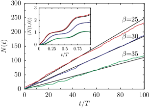
Figure 1: The number of transitions $N(t)$ accumulated from $0$ up to time $t$ as a function of $t$ for simulations with the driving strength $A=0.1$, driving period $\Omega=10^{-3}$, and inverse temperatures $\beta=25$ (red), $30$ (blue) and $35$ (green) is depicted together with the average behavior (black straight lines) resulting from the two-state theory, see eq. (15). Note that the observed deviations apparently are smallest for the middle inverse temperature $\beta=30$. The mean value $\langle N(t)\rangle$ obtained from the simulations as the average over all available periods is compared with the theoretical prediction in eq. (15).

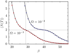
Figure 2: The average number of transitions $\langle N(T)\rangle\equiv\langle N(T,0)\rangle$ occurring in one period is shown as a function of the inverse temperature for the two driving frequencies $\Omega=10^{-3}$ (red $\times$) and $10^{-4}$ (blue $+$) and the driving strength $A=0.1$. The symbols representing the results of the simulations nicely fall onto the respective theoretical curves from equation (15) shown as black lines. At the temperatures (thin black vertical lines) where $\langle N(T)\rangle$ assume the value 2 indicated by the thin black horizontal line, the dynamics is optimally synchronized with the external driving force. For the smaller frequency the average number of transitions flattens around this optimal temperature value indicating a tighter locking of the transitions with the external driving force.

In Fig. 2 the estimated value of this number is compared with the two-state model prediction as a function of $\beta$. The agreement between theory and simulations is excellent even for the relatively high temperature values and corresponding low transition barriers for the values of $\beta<25$. The average number of transitions monotonically decreases with falling temperature. At the temperature where $\langle N(T+s,s)\rangle^{\text{as}}=2$ the system is optimally synchronized with the driving force in the sense that the Rice phase increases on average by $2\pi$ per period of the driving force. This optimal temperature depends on the driving frequency and becomes lowered for slower driving. In the vicinity of the optimal temperature the decrease of $\langle N(T+s,s)\rangle^{\text{as}}$ with inverse temperature is smallest. The emerging flat region resembles the locking of a driven nonlinear oscillator and becomes more pronounced for smaller driving frequencies.

The fluctuations of the number of transitions $\delta N(t)\equiv N(t,0)-\langle N(t,0)\rangle$ for times up to $t=500T$ in a single simulation together with the theoretical average following from eq. (22) are shown in Fig. 4.

Figure 3: The fluctuations of the number of transitions $\delta N(t)$ for $A=0.1$, $\Omega=10^{-3}$ and $\beta=35$ (jagged line) appears as diffusive. The smooth curve depicts the root behavior of the diffusion law $\langle\delta N^{2}(t)\rangle=2D(0)t$ with the diffusion constant $D(0)=\langle\delta N^{2}(T,0)\rangle/(2T)=5.36\times 10^{-5}$ resulting from the two-state model, see eq. (25).

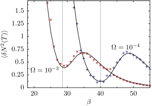
Figure 4: The variance of the number of transitions $\langle\delta N^{2}(T)\rangle\equiv\langle\delta N^{2}(T,0)\rangle$ in one period is shown as a function of the inverse temperature. The symbols are the same as in Fig. 2, the solid lines display equation (22). Note that $\langle\delta N^{2}(T)\rangle$ is proportional to the diffusion constant of the Rice phase. The vertical thin black lines indicate the optimal inverse temperatures as found from the synchronization of the averaged phase (see Fig. 2). They coincide remarkably well with the positions of the minima of $\langle\delta N^{2}(T)\rangle$. So we find that at the optimal temperature also the fluctuations of the number of transitions and consequently of the generalized Rice phase are suppressed.

The average behavior is characterized by the number fluctuations per period $\delta N^{2}(T,0)$. This quantity was estimated from the simulations as a function of the inverse temperature. In Fig. 4 we compare the prediction of the two-state model, see eq. (22) with numerics. These number fluctuations exhibit a local minimum very close to the optimal temperature where two transitions per period occur on average, see Figs. 2 and 4. This minimum is more pronounced for the lower driving frequency. The fluctuations of the Rice phase also assume a minimum at this optimal temperature. This means that the phase diffusion is minimal at this temperature.

For the Fano factor $F(0)$ we obtain an absolute minimum near the optimal temperature, see Fig. 5. For higher temperatures the Fano factor may become larger than one, whereas it approaches the Poissonian value $F=1$ for low temperatures because then, transitions become very rare and independent from each other. Also here, theory and simulations agree indeed very well.

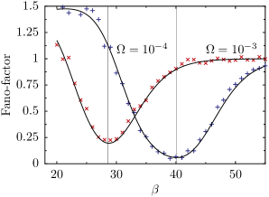
Figure 5: As a relative measure of number and phase fluctuations, the Fano factor $F=F(0)$ from equation (26) is shown as a function of the inverse temperature. Symbols are the same as in Fig. 2. The minimum positions of the Fano factor again nicely coincide with the optimal temperature values indicated by the thin black lines. With decreasing frequency these minima move to lower temperatures and become broader and deeper. For sufficiently low temperatures the transitions become very rare and almost Poissonian leading to the asymptotic low temperature limit $F=1$.

Next, we consider the probabilities $P(n)=P(n;T,0)$ for finding $N(T,0)=n$ transitions per period in the asymptotic, periodic limit. For this purpose we count the number $k$ of transitions within each period $[nT,(n+1)T)$ and determine their relative frequency occurring in a simulation. A comparison with the prediction of the two-state model determined from the numerical integration of eq. (3) and from eq. (30) is collected in Fig. 6 for different temperature values. The agreement between simulations and theory is within the expected statistical accuracy. For large temperatures there is a rather broad distribution of $n$-values around a most probable value $n^{*}$. With decreasing temperature, the most probable value moves to smaller numbers whereby the width of the distribution shrinks. Once $n^{*}=2$ the probability $P(2)$ further increases at the cost of the other $k$ values with decreasing temperature until $k=0$ gains the full weight in the limit of low temperatures.

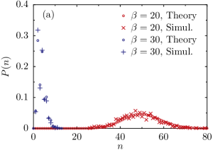
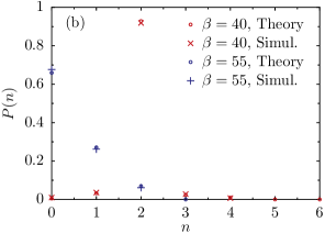
Figure 6: The probabilities $P(n)=P(n;T,0)$ are shown for the driving the driving strength $A=0.1$ and the driving frequency $\Omega=10^{-4}$; for two temperatures that are higher than the optimal one corresponding to $\beta\approx 40$ in panel (a) and and for the optimal and a lower temperature in panel (b). As one expects for a good synchronization of the system with the driving force at the optimal temperature one finds two transitions per period with about $90\%$ of the total weight. For high temperatures the distribution becomes rather broad with a maximum at some large number of transitions. On the contrary, for low temperatures the probability is largest at $n=0$ and decreases with $n$. The agreement of the two-state theory resulting from equation (30) with the simulations is remarkably good.

The degree of synchronization of the continuous bistable dynamics with the external driving force can be characterized by the value of the probability $P(2)$. As a function of the inverse temperature $\beta$ it has a maximum close to the corresponding optimal temperature, see Fig. 8. For the longer driving period the maximum is at a lower temperature and its value is higher. Fig. 8 depicts $P(2)$ as a function of the frequency at a fixed temperature. It has a maximum at some optimal value of the frequency.

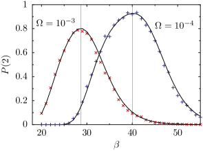
Figure 7: The probability $P(2)=P(n=2;T,0)$ for two transitions within one period is shown as a function of the inverse temperature $\beta$. Results from the simulations are depicted by red ($\times$) and blue ($+$) crosses for two frequencies. They agree well with the respective theoretical predictions of the two-state theory resulting from equation (30) (solid lines). The probabilities show the typical stochastic resonance behavior with a maximum very close to the optimal temperature. As for the minimum of the Fano factor, this maximum is more pronounced at the lower driving frequency.

Figure 8: The probability $P(2)=P(n=2;T,0)$ (see equation (30)) for two transitions within one period is shown as a function of the frequency at the inverse temperature $\beta=35$. It also shows a resonance like behavior with a maximum at an optimal frequency.

Finally, we come to the residence time distributions which can be estimated from histograms of the simulated data. In the Fig. 9 these histograms are compared with the results of the two-state model. Theory and simulations are in good agreement and show a transition from a multi-modal distribution with peaks at odd multiples of half the period to a mono-modal distribution at zero as one would expect. At stochastic resonance taking place at the inverse temperature $\beta\approx 40$ the distribution is also mono-modal with its maximum close to half the period.

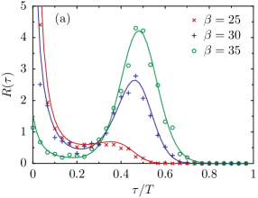
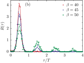
Figure 9: Residence time distributions for either of the two states are shown for $\Omega=10^{-4}$ and different values of the temperature. Theoretical results obtained from (eq. 31) are displayed as solid lines, estimates from the simulations as symbols. In panel (a) $R(\tau)$ is shown for higher temperatures and in panel (b) for the optimal and lower than optimal temperatures. The peak structure and its temperature dependence is in complete agreement with previous findings, see Ref. [1].

5 Discussion and conclusions

In this work we investigated the statistics of transitions between the two states of a periodically driven overdamped bistable Brownian oscillator. We compared results from extensive numerical simulations with theoretical predictions of a discrete Markovian two-state model with time-dependent rates. For the studied slow driving frequencies the rates can be taken as the adiabatic, or frozen, rates. Although the minimal barriers separating the states from each other may become rather small measured in units of the thermal energy ($\beta V_{\text{min}}\approx 4$ for the lowest inverse temperature $\beta=20$) we did not take into account finite barrier corrections for the rates and still obtained very good agreement for all considered quantities even at the highest chosen temperatures. We considered different quantities from the counting statistics of transitions such as the average and variance, as well as the probability of a given number of transitions in one period. These quantities are directly related to the average Rice phase, its diffusion and the probability of a given increase of this phase. We note that, apart from the average phase, these quantities depend on the position of the chosen period for which we took $s=0$ as the starting time. A different, more sophisticated, way of analyzing the counting statistics would have been to position the averaging window of the length of a period such that the variance of the number of transitions is minimal. But already with the present simpler method we could detect significant signatures of synchronization in a noisy nonlinear system such as the locking of frequency and phase which both occur at basically the same parameter values.

The novel analytical expression for the residence time distribution derived for the two-state model also agrees very well with the simulation results.

References

References

- [1] Gammaitoni L, Hänggi P, Jung P and Marchesoni F 1998 Rev. Mod. Phys. 70 223
-
[2]
Reimann P 2002 Phys. Rep. 361 57
Astumian R D and Hänggi P 2002 Phys. Today 55(11) 33
Reimann P and Hänggi P 2002 Appl. Phys. A 75 169 -
[3]
Rozenfeld R, Freund J A, Neiman A and Schimansky-Geier
L 2001 Phys. Rev. E 64 051107
Freund J A, Neiman A B and Schimansky-Geier L 2000 Europhys. Lett. 50 8
Park K, Lai YC, Liu ZH and Nachman A 2004 Phys. Lett. A 326 391 -
[4]
Callenbach L, Hänggi P, Linz S J, Freund J A and
Schimansky-Geier L 2002 Phys. Rev. E 65 051110
Freund J A, Schimansky-Geier L and Hänggi P 2003 Chaos 13 225 - [5] Hänggi P and Thomas H 1982 Phys. Rep. 88 207
- [6] Jung P and Hänggi P 1990 Phys. Rev. A 41 2977 Jung P 1993 Phys. Rep. 234 175
- [7] Lehmann J, Reimann P and Hänggi P 2000 Phys. Rev. Lett. 84 1639 Reimann P, Lehmann J and Hänggi P 2000 Phys. Rev. E 62 6282 Lehmann J, Reimann P and Hänggi P 2003 Phys. Status Solidi B 237 53
- [8] Schindler M, Talkner P and Hänggi P 2004 Phys. Rev. Lett. 93 048102
- [9] McNamara B and Wiesenfeld K 1989 Phys. Rev. A 39 4854
-
[10]
Shneidman V A, Jung P and Hänggi P 1994 Phys. Rev. Lett. 72 2682
Shneidman V A, Jung P and Hänggi P 1994 Europhys. Lett. 26 571
Casado-Pascual J, Gomez-Ordonez J, Morillo M and Hänggi P 2003 Phys. Rev. Lett. 91 210601 - [11] Talkner P and Łuczka J 2004 Phys. Rev. E 69 046109
- [12] Rice S O Mathematical Analysis of Random Noise. In Wax N (ed) 1954 Selected Papers on Noise and Stochastic Processes (New York: Dover) p 133
- [13] Talkner P 2003 Physica A 325 124
- [14] Gammaitoni L, Marchesoni F and Santucci S 1995 Phys. Rev. Lett. 74 1052
-
[15]
Fano U 1947 Phys. Rev. 72 26
Shuai J W and Jung P 2003 Fluct. Noise Lett. 2 L139 - [16] Hänggi P, Talkner P and Borkovec M 1990 Rev. Mod. Phys. 62 251
- [17] Talkner P 1999 New J. Phys. 1 4
- [18] Cox D R and Miller H D 1972 The Theory of Stochastic Processes (London: Chapman and Hall)
- [19] Stratonovich R L 1963 Topics in the Theory of Random Noise Vol. 1 (New York: Gordon and Breach)
- [20] Löfstedt R L and Coppersmith S N 1994 Phys. Rev. E 49 4821
- [21] Choi M H, Fox R F and Jung P 1998 Phys. Rev. E 57, 6335
- [22] Matsumoto M and Nishimura T 1998 ACM Trans. Modeling and Comp. Sim. 8 3
-
[23]
Lüscher M 1994 Comput. Phys. Commun. 79 100
L’Ecuyer P 1996 Math. Comput. 65 203