GPS radio occultation with GRACE: Atmospheric profiling utilizing the zero difference technique

Abstract

Radio occultation events recorded on 28–29 July 2004 by a GPS receiver aboard the GRACE-B satellite are analyzed. The stability of the receiver clock allows for the derivation of excess phase profiles using a zero difference technique, rendering the calibration procedure with concurrent observations of a reference GPS satellite obsolete. 101 refractivity profiles obtained by zero differencing and 96 profiles calculated with an improved single difference method are compared with co-located ECMWF meteorological analyses. Good agreement is found at altitudes between 5 and 30 km with an average fractional refractivity deviation below 1% and a standard deviation of 2–3%. Results from end-to-end simulations are consistent with these observations.

BEYERLE ET AL. GPS OCCULTATION USING ZERO DIFFERENCING G. Beyerle, S. Heise, G. Michalak, Ch. Reigber, T. Schmidt, J. Wickert, GeoForschungsZentrum Potsdam (GFZ), Department 1, Geodesy and Remote Sensing, Telegrafenberg, D-14473 Potsdam, Germany (e-mail: gbeyerle@gfz-potsdam.de)

Gindraft=false

1 Introduction

In recent years atmospheric sounding by space-based Global Positioning System (GPS) radio occultation (RO) is considered a valuable data source for numerical weather prediction and climate change studies. From 1995 to 1997 the proof-of-concept GPS/MET mission performed a series of successful measurement campaigns (Rocken et al., 1997); since 2001 a RO instrument operates aboard the CHAMP (CHAllenging Minisatellite Payload) (Reigber et al., 2004) satellite.

During an occultation event the RO receiver aboard the low Earth orbiting (LEO) spacecraft records dual-frequency signals transmitted from a GPS satellite setting behind the horizon. Voltage signal-to-noise ratios ($S\!N\!R_{v}$) and carrier phases at the two GPS L-band frequencies $f_{1}=1.57542$ GHz (L1) and $f_{2}=1.2276$ GHz (L2) are tracked with a sampling frequency of typically 50 Hz. The ionosphere and neutral atmosphere induce optical path length deviations from the geometrical distance between transmitter and receiver. These deviations are denoted as excess phase paths $\chi$ and are related to the ray bending angle $\alpha$ as a function of impact parameter $p$. From $\alpha(p)$ the atmospheric refractivity profile $N(z)=(n(z)-1)\cdot 10^{6}$ is derived, where $n(z)$ denotes the real part of the atmospheric refractive index at altitude $z$ (Kursinski et al., 1997; Hajj et al., 2002).

GPS/MET observations were analyzed with a double difference method to correct for clock errors of the GPS transmitters and the receiver aboard the LEO satellite (Rocken et al., 1997). Since deactivation of Selective Availability (S/A), an intentional degradation of broadcast ephemeris data, on 2 May 2000, the GPS clock errors are reduced by orders of magnitude. Without S/A GPS clocks are sufficiently stable to replace double differencing by the single difference technique thereby eliminating the need for concurrent high-rate ground station observations (Wickert et al., 2002).

On 28–29 July 2004 the GPS RO receiver aboard the GRACE-B satellite, the second of the two GRACE satellites (Tapley et al., 2004), was activated for 25 hours to test the receiver’s occultation mode (Wickert et al., 2005). The GRACE-B receiver clock time was adjusted to GPS coordinate time only once during the measurement period. Thus, the GRACE-B clock solutions can be interpolated from the precise orbit determination’s (POD) temporal resolution of 30 s to the occultation receiver’s resolution of 20 ms and the excess phase path is obtained without simultaneous observations of a reference GPS satellite (zero differencing).

2 Methodology and Data Analysis

The L1 and L2 signals transmitted by the occulting GPS satellite are recorded by the receiver’s signal tracking phase-locked loops. Their numerically-controlled oscillators (NCOs) are phase-locked to the signal carriers transmitted by the GPS satellite which in turn are phase-locked to the GPS transmitter clock. We may regard the NCOs as clocks that are synchronized to the transmitter clock of the occulting satellite. The occulting GPS clock time, as recorded by the receiver NCO, is denoted by $\hat{t}^{O}_{k}$. ($k=1$ for L1, $k=2$ for L2; though, in the following the subscript $k$ is omitted.) During an occultation event the receiver measures both $\hat{t}^{O}$ and the corresponding LEO clock time $\hat{t}^{L}$.

2.1 Zero and Single Differencing Methods

Since the GPS and LEO satellites move within Earth’s gravitational potential, the proper time $\bar{t}$, the coordinate time $t$ and the clock time $\hat{t}$ in general will not agree. In order to extract the excess phase paths $\chi(t)$ from the measurements $L^{OL}\equiv c\,(\hat{t}^{L}-\hat{t}^{O})$, the LEO clock corrections $(\hat{t}^{L}-{t}^{L})$ and the occulting GPS clock corrections $(\hat{t}^{O}-{t}^{O})$ have to be taken into account (Hajj et al., 2002). Here, $c$ denotes the velocity of light in vacuum. We note that both, $(\hat{t}^{L}-{t}^{L})$ and $(\hat{t}^{O}-{t}^{O})$, include relativistic effects relating coordinate time to proper time. Thus, the zero differencing (ZD) equation is

$${t}^{L}-{t}^{O}=\frac{1}{c}\,L^{OL}-(\hat{t}^{L}-{t}^{L})-({t}^{O}-\hat{t}^{O})\;.$$ (1)

The left hand side of Eqn. 1 contains the excess phase path $\chi$ through

$${t}^{L}-{t}^{O} \approx \frac{1}{c}\,\left(d^{OL}+\chi\right)$$ (2)

where contributions from the gravitational time delay are neglected (Hajj et al., 2002) and $d^{OL}\equiv|\vec{r}^{O}-\vec{r}^{L}|$. The positions of the occulting GPS and the LEO satellite, $\vec{r}^{\,O}$ and $\vec{r}^{\,L}$, and their clock corrections, $(\hat{t}^{O}-{t}^{O})$ and $(\hat{t}^{L}-{t}^{L})$, are obtained from the POD (König et al., 2004). CHAMP’s and GRACE-B’s orbits and clock solutions are provided at a temporal resolution of 30 s.

GRACE-B’s receiver clock is adjusted to GPS coordinate time only once during the 25 hour measurement period on 28 July 16:24 UTC. The difference between clock time and coordinate time, $(\hat{t}^{L}-{t}^{L})$, at the required temporal resolution of 20 ms could therefore successfully be interpolated from the 30 s clock solutions. The receiver clock aboard CHAMP, on the other hand, is adjusted once per second to achieve a 1 $\mu$s maximum deviation with respect to coordinate time. (See discussion of Fig. 2 below.) These adjustments introduce discontinuities that cannot be corrected for on the basis of the 30 s clock solutions and require the simultaneous observation of a referencing GPS satellite (single differencing (SD))

$$t^{L}-t^{O} = \frac{1}{c}\,(L^{OL}-L^{RL}_{c})+({t}^{L}-{t}^{R})+({t}^{R}-\hat{t}^{R})-({t}^{O}-\hat{t}^{O})$$ (3)

with superscript $R$ indicating the reference satellite (Wickert et al., 2002). The reference link observation corrected for ionospheric signal propagation, $L^{RL}_{c}$, is calculated from

$$L^{RL}_{c}\equiv c_{1}\,L^{RL}_{L1}-c_{2}\,L^{RL}_{L2}\;.$$ (4)

with parameters $c_{1}$ and $c_{2}$ defined as $c_{i}=(f_{i})^{2}/[(f_{1})^{2}-(f_{2})^{2}]$, $i=1,2$.

GFZ’s operational RO processing system (Wickert et al., 2004) improves the ionospheric correction of the reference link observations (Eqn. 4) by assuming that quiet ionospheric conditions prevail (modified single differencing, in the following abbreviated as SDM). Within the SDM approach $L^{RL}_{c}$ is replaced by

$$\tilde{L}^{RL}_{c}\equiv L^{RL}_{L1}+c_{2}\,\langle L^{RL}_{L1}-L^{RL}_{L2}\rangle$$ (5)

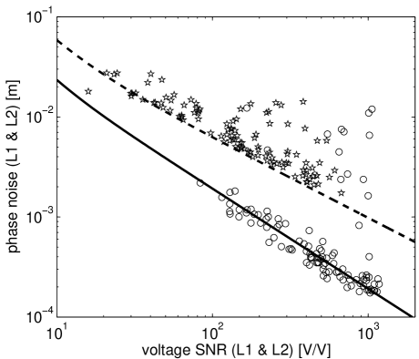
Figure 1: Carrier phase noise extracted from the reference link observations as a function of voltage $S\!N\!R_{v}$. The L1 and L2 observations extracted from 109 reference link profiles are marked as circles and stars, respectively. The L1 phase noise (full line) is calculated from Eqn. 6 with $T=20$ ms and $B_{w}=20$ Hz; the corresponding L2 noise (dashed line) is a heuristic parameterization since additional losses from semi-codeless or codeless L2 tracking are not taken into account by Eqn. 6.

where $\langle\cdot\rangle$ denotes a smoothing (low-pass) filter. Since the noise level of $L^{RL}_{L2}$ is much larger than the noise level of $L^{RL}_{L1}$ (see Fig. 1) the filter effectively reduces the L2 noise.

2.2 Comparison with ECMWF

The observed GRACE refractivity profiles are intercompared with meteorological analysis results provided by the European Centre for Medium-Range Weather Forecasts (ECMWF). Pressure and temperature values from the ECMWF fields are calculated by linear interpolation between grid points (0.5${}^{\circ}\times 0.5^{\circ}$ resolution). Linear interpolation in time is performed between 6 h analyses fields. The comparison between RO observation and meteorological analysis is performed on the 60 ECMWF model levels ranging from the ground surface up to 0.1 hPa (about 60 km altitude) after converting the pressure levels to height coordinates. Vertical spacing of the model grid points increases from about 200 m at 1 km altitude to about 700 m at 10 km altitude.

2.3 Simulation Study

We interpret the GRACE-B observations using results from end-to-end simulations. The refractivity field is assumed to be spherically symmetric and calculated from the corresponding ECWMF profile; electron densities are modelled using the Parameterized Ionospheric Model (PIM) (Daniell et al., 1995). The occultation events are simulated with circular approximations of the true GRACE-B and GPS satellite orbits. Signal amplitudes and carrier phases on the occultation link are calculated from bending angles with the inverse CT technique (Gorbunov, 2003) modified for circular orbits (inverse FSI or CT2 method). The amplitude is normalized to the observation averaged over the first 10 s of the occultation. The reference link data are assumed to be multipath-free and the carrier phases are determined using geometric optics, their signal amplitudes are taken to be constant. Again, their magnitude is extracted from the observation. On both links ray bending due to the ionosphere and neutral atmosphere is taken into account.

In principle, carrier tracking loop errors as well as clock instabilities and ionospheric disturbances contribute to the uncertainties of the observations $L^{OL}$ and $L^{RL}$. For a given amplitude $S\!N\!R_{v}$ the tracking loop phase noise $\sigma_{c}$ can be estimated from (Ward, 1996)

$$\sigma_{c}=\frac{\lambda}{2\pi}\,\sqrt{\frac{2\,B_{w}\,1\,\textrm{s}}{(S\!N\!R_{v})^{2}}\,\left(1+\frac{1\,\textrm{s}}{(S\!N\!R_{v})^{2}\,T}\right)}$$ (6)

with carrier wavelength $\lambda$, sampling time $T$ and carrier loop bandwidth $B_{w}$.

The simulated L1 phase noise is calculated from Eqn. 6 using $T=20$ ms and $B_{w}=20$ Hz, since this parametrization is in approximate agreement with the observed $L^{RL}_{L1}$ noise levels which are plotted in Fig. 1 (circles). The full line marks the result from Eqn. 6. The corresponding L2 noise values, however, estimated from Eqn. 6 significantly underestimate the observations since additional losses from semi-codeless or codeless L2 tracking are not taken into account by Eqn. 6. A heuristic parametrization is therefore used to simulate the L2 phase noise (dashed line in Fig. 1).

The uncertainties of both observations, $L^{RL}_{L1}$ and $L^{RL}_{L2}$, exhibit a distinct dependency on $S\!N\!R_{v}$ (Fig. 1). Since the clock error is expected to be independent of $S\!N\!R_{v}$ we conclude from Fig. 1 that tracking loop errors dominate the clock uncertainties. Enhanced noise values in some of the observations are presumably attributed to ionospheric disturbances. From the simulated $S\!N\!R_{v}(t)$ and $\chi(t)$ data bending angle profiles are reconstructed using the FSI method (Jensen et al., 2003) and (above 20 km altitude) using the geometric optics method. Finally, refractivity profiles are retrieved by Abel-transforming (Fjeldbo et al., 1971) the bending angle profiles thereby closing the simulation loop.

3 Discussion

Between 6:03 UTC on 28 July 2004 and 7:09 UTC on 29 July 2004 the GPS receiver aboard GRACE-B was activated to test occultation measurement mode. During these 25 hours the receiver recorded 109 occultation events lasting longer than 40 s; 101 events could be successfully converted to atmospheric refractivity profiles with ZD and SDM processing, 8 were removed as outliers. A profile is regarded as outlier if the fractional refractivity error with respect to ECMWF exceeds 10% at altitudes above 10 km. The corresponding yield for SD is 96 profiles.

From the reference link observations $L^{RL}$ the difference between receiver clock time and proper time, $(\hat{t}^{L}-\bar{t}^{L})$, can be estimated assuming quiet ionospheric conditions (Wickert et al., 2002). Its temporal evolution, $\Delta(\hat{t}^{L}-\bar{t}^{L})/T$, extracted from the first GRACE-B occultation measurement on 28 July 2004, 6:10 UTC at 55.3^∘N, 22.3^∘E, is plotted in Fig. 2, bottom panel, black line. Here, $\Delta(x_{n})\equiv x_{n+1}-x_{n}$ denotes the forward difference operator and the sampling rate is $T=20$ ms. The mean clock drift of $31.3347\pm 0.6305$ ns/s is consistent with a $31.3338$ ns/s mean drift obtained from GRACE-B precise orbit calculations (white line).

For comparison the top panel of Fig. 2 shows an occultation event recorded by CHAMP on the same day, 0:18 UTC at 69.4^∘N, 12.5^∘W. The CHAMP clock drift ($-1.0642\pm 8.5187$ ns/s) exhibits periodic discontinuities of about $10$ ns/s about every 18 s; in addition, the CHAMP clock is adjusted every second in order to meet the design specification of 1 $\mu$s absolute time signal error with respect to coordinate time. These discontinuities cannot be modelled from the 30 s POD data eliminating at present the possibility of zero differencing with CHAMP. Since the data sets shown in Fig. 2 are extracted from reference link observations, the random components contain contributions from the ionosphere as well as the tracking loops and should not be interpreted as clock noise.

The mean fractional refractivity error $\langle(N_{obs}-N_{met})/N_{met}\rangle$ derived from the GRACE-B observations is plotted in Fig. 3 (left panel), where $N_{obs}$ and $N_{met}$ denote the observed and ECMWF refractivities, respectively. The 1-$\sigma$ standard deviations are marked as thin lines. The number of extracted data points as a function of altitude is plotted in the right panel.

The ZD results are characterized by smaller standard deviations at altitudes below 20 km since noise contributions from the reference link are present in the SD, but not in the ZD excess phases. Above 20 km multipath is assumed to be negligible and bending angles are calculated using geometric optics. In addition, the SDM results are marked by crosses in the left panel of Fig. 3. The almost perfect agreement with the ZD profiles, both in terms of bias (crosses) and standard deviation (not shown), emphasizes the impact of the respective ionospheric correction procedure (Eqn. 4 vs. Eqn. 5) on the tropospheric retrieval results.

Fig. 3 suggests that ZD processing reduces the lower tropospheric refractivity bias compared to the SD results. At low $S\!N\!R_{v}$ substantial phase noise contributions are present in the excess phase path profile $\chi(t)$ thereby degrading the radioholographic interference patterns encoded in $\chi(t)$. These patterns originate from interfering rays associated with large negative vertical refractivity gradients that are caused by humidity layers in the lower troposphere. From the degraded interference patterns the FSI algorithm underestimates the large bending angles produced by the vertical refractivity gradients leading to smaller refractivities and, ultimately, a negative bias with respect to ECMWF.

We substantiate our interpretation of the difference between ZD and SD data with simulation results shown in Fig. 4. We note that the non-zero mean fractional refractivity error and standard deviation is caused by including L1/L2 carrier phase noise within the simulation. Above 20 km altitude the bending angles derived from the FSI are replaced by the values obtained from the geometric optics method, since the occurrence of multipath ray propagation in the stratosphere can be excluded. The simulations reproduce the over-all differences between the observed ZD and SD refractivities (Fig. 3) as well as an (albeit smaller) bias between the two data sets at altitudes below 10 km. An additional SD simulation was conducted with the noise level of the reference link observations reduced to zero. Since the result (marked by crosses in Fig. 4) is in excellent agreement with the ZD profile throughout the full altitude range, the observed bias between the ZD and SD results in the lower troposphere is evidently caused by the reference link phase noise.

4 Conclusion

First radio occultation events observed by the GRACE-B satellite are successfully analyzed using zero differencing. In the upper troposphere and lower stratosphere the refractivities derived from zero and single differencing are in good agreement with the corresponding ECMWF meteorological analyses. Zero differencing allows for a reduction in the amount of down-link data. More significantly, zero differencing reduces the noise level on the excess phase paths and thereby yields less-biased refractivities within regions of multipath signal propagation in the lower troposphere compared to single differencing. However, for quiet ionospheric conditions a modified single differencing method can be applied producing refractivities that are in excellent agreement with the zero differencing results.

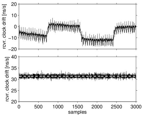
Figure 2: Receiver clock drift derived from GRACE-B and CHAMP reference link data. Top: receiver clock drift observed in a CHAMP occultation event on 28 July 2004, 0:18 UTC at 69.4^∘N, 12.5^∘W. Bottom: clock drift observed in a GRACE occultation event on 28 July 2004, 6:41 UTC at 66.6^∘S, 13.9^∘E (black). Note the change in vertical scale.

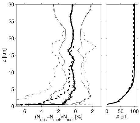
Figure 3: Left: Mean fractional refractivity deviation between GRACE observations and ECMWF analyses. The data set comprises 101 zero differencing (solid line) and 96 single differencing (dashed line) results. Thin lines indicate the 1-$\sigma$ standard deviations. Retrieval results from modified single differencing are marked as crosses. Right: number of data points retrieved as a function of altitude.

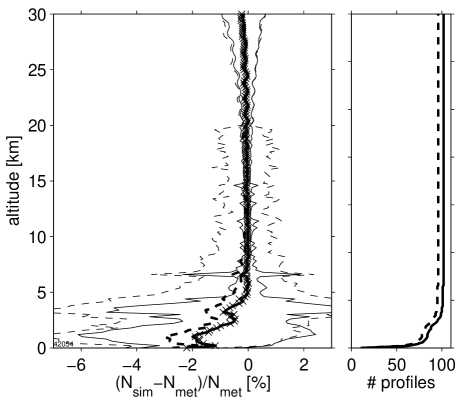
Figure 4: Same as Fig. 3, except that results from end-to-end simulations are shown. Left: the mean error for ZD and SD processing are plotted as thick solid and dashed lines, respectively. Thin lines indicate the 1-$\sigma$ standard deviations. The result obtained from a SD simulation with noise-free reference link phase observations (crosses) is in almost perfect agreement with the ZD result. Right: number of data points retrieved as a function of altitude.