Non-linear plane perturbation in a
non-ohmic/ohmic fluid interface in a vertical electric field

Abstract

The stability of a non-ohmic/ohmic fluid interface in the presence of a constant gravitational field and stressed by a vertical stationary electric field with unipolar injection is studied, focusing on the destabilising action of the electric pressure when charge relaxation effects can be ignored. We use a hydraulic model, whose static equilibrium condition is written and analysed as a function of the ohmic fluid conductivity when subjected to a non-linear perturbation. The combined action of the polarization and free interfacial charges on the pressure instability mechanism is also analysed. The results show some important peculiarities of the fluid interface behaviour in the presence of a stationary space charge distribution generated by unipolar injection in the non-ohmic fluid.

I Introduction

If a stationary electric field ${\mathbf{E}}$, parallel to a constant gravitational field ${\mathbf{g}}$, is applied on a system composed by two immiscible fluids with different mass densities, the interface between them should rest, in the state of equilibrium, completely plane and perpendicular to the fields and eventually subjected to the destabilization when the corresponding electric field is strong enough. In general, in this paper, the term non-ohmic/ohmic, for example, refers to an interface where the lower fluid layer is ohmic.

Taylor and McEwan Taylor and McEwan (1965) studied the static equilibrium of this system in the case of a non-conducting/conducting ohmic interface and determined the instability criterion in a linear theory. In this case, the stress acting on the interface is acting only in its normal direction: we say that the instability is due to a pressure mechanism. Melcher & Smith Melcher and Jr. (1969) studied the stability of an ohmic/ohmic interface stressed by a vertical electric field in a more general linear theory considering all possible conductivity values of both fluids (and also other physical properties involved, such as viscosity, etc.), including charge relaxation effects under these conditions. In this work, shear stresses are involved and hence overstability Chandrasekhar (1961) and surface charge convection may occur. We say that in this case the instability is due to the convective mechanism. (Please note that in this case convection is due to surface charge not to volume charge, like in the electrohydrodynamic instability due to unipolar injection in an insulating liquid layer Atten and Moreau (1972); Lacroix et al. (1975)).

Some recent work on this problem has investigated a non-ohmic/ohmic fluid interface when the non-ohmic layer is subjected to unipolar injection Atten and Koulova-Nenova (1999); Vega and Pérez (2002a). These works are motivated because in certain experimental systems an electrode may act not only as a voltage source (a surface charge source, in the end) but also as a space charge source Atten and Moreau (1972). Melcher & Schwartz Melcher and Jr. (1968) noticed that an electrode may cause, if in contact with a very low conducting fluid, dielectrical breakage and generate a stationary electric field with a space charge distribution in the non-ohmic part of the system. This makes the coupling of the electric field with mechanical fluid equations very different from that occurring in the classical studies of ohmic/ohmic fluid interfaces. A clear example is the experiment by Koulova-Nenova, Malraison & Atten Koulova-Nenova, Malraison, and Atten (1996), where a moderate injection in a liquid mixture of ciclohexane with TiAP salt Denat (1982) was produced. They observed that unipolar injection from the electrode may produce not only convection in the bulk of the fluid but also an interfacial instability similar to that occurring in the absence of space charge Taylor and McEwan (1965) but with a peculiarity: the voltage thresholds for instability are systematically reduced by 1/3. The complete linear theory for a non-ohmic/ohmic interface is presented in the previous work by Vega & Pérez Vega and Pérez (2002a), where a transition region in the critical behaviour of the interface has been found. This region marks the conducting-to-insulating transition in the behaviour of the non-ohmic/ohmic interface. In fact, the existence of this transition region implies that the dynamics of the same non-ohmic/ohmic interface subjected to unipolar injection may behave like in an ohmic/ohmic interface in which the lower layer is the most conducting, but also like in an ohmic/ohmic interface in which the lower layer is the least conducting (insulating behaviour). However, by definition, in the non-ohmic/ohmic interface the lower layer is always the most conducting. The apparent contradiction comes from the fact that, under unipolar injection, the electric conduction in the non-ohmic layer may be actually more ”effective” than the ohmic conduction in the lower layer, depending on the value of the applied electric potential. This causes the mechanics of the fluid interface to be much more complex when there is injection.

The purpose of this paper is to demonstrate that this complexity appears already in the electric pressure instability mechanism; i.e., the static interfacial equilibrium between electric and gravitational forces. In order to make clear an intuitive visualization of this equilibrium, a hydraulic model is developed (figure 1). The system described in the model is not that of an infinite fluid interface and thus the results are not, in general, quantitatively applicable to the infinite interface problem. However, as it will be shown, the results of the hydraulic model can account for the same transition region described above Vega and Pérez (2002a). Thus, the hydraulic model yields a qualitatively analogous description of the corresponding problem in the infinite interface. But the results are not only restricted to comparison of results in a previous work Vega and Pérez (2002a). They also provide the following additional inputs: a) identification of the mechanism that causes the transition region to appear (electric pressure due to polarization charges) and precise determination of the transition region, and b) observation of this transition as a function of the perturbation amplitude (not only as a function of conductivity as previously detected Vega and Pérez (2002a)). As we will see this implies that, once the instability begins, an interface with a very conducting lower layer may be stabilized in states with non-zero perturbation amplitudes. This behaviour differs from that observed in the purely ohmic case Taylor and McEwan (1965); Koulova-Nenova et al. (1996), where the interfacial perturbation grows continually because the electrical pressure mechanism is always actively pulling up or pushing down the interface.

The interest of this problem is due to the original behaviour of this putative fluid interface and its possible industrial applications. For example, the formation of stable metallic liquid points when the interface changes from conducting (the electric pressure has opposite sign to the applied field) to non-conducting behaviour (the electric pressure keeps the same sign that the applied field) in a perturbed state could be used to make ion sources.

The possibility of producing ion sources by manipulating a fluid interface with electric fields motivated the work by Néron de Surgy de Surgy (1995), who extended the original work by Taylor and McEwan Taylor and McEwan (1965) introducing a non-linear perturbation in a non-conducting/conducting ohmic fluid interface, but always without injection. The results proved theoretically that a metallic liquid can never develop stable points, independently of the geometry of the system. However, in some rare cases he experimentally observed stable metallic points, which Néron indicated could be due to impurities in the liquid. We suggest in this paper that this is related to an injection from the metallic liquid points to the air.

In §II.1 we describe the hydraulic model and find its non-linear stability condition. In §II.2 we find the difference between the stability condition in the hydraulic model and the one found for the infinite interface in a previous work Vega and Pérez (2002a). The effect of the combined action of polarization and free surface charges will be explained in §II.3. In §II.4 we introduce the reduced critical parameter $U_{NL}$ and the possible general behaviours of the non-linear critical curves are described. Finally, in §III and §IV we present the results of the hydraulic model in the cases of an ohmic/ohmic interface and the non-ohmic/ohmic interface, respectively. Although the purely ohmic interface has been studied extensively Taylor and McEwan (1965); Melcher (1963); de Surgy (1995), the results of §III are interesting to make evident the new perspective gained with the hydraulic model.

II Hydraulic model

II.1 The system and the equilibrium equation

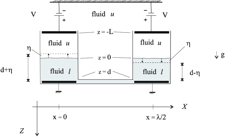
Figure 1: The system studied. A plane perturbation of amplitude $\eta$ is introduced in such a way that the interface level is raised in the cylinder centered in $x=0$ and lowered in the other cylinder (which is centered at $x=\lambda/2$).

The system (figure 1) consists of two identical rigid cylinders with parallel axes, connected to each other through a thin horizontal cylindrical pipe at their base. The system is in a constant gravitational field with a constant acceleration $\mathbf{g}=g\mathbf{u}_{z}$ (this field acts in a direction called ”vertical”; thus, its perpendicular plane defines the horizontal directions). The system is immersed in a fluid u, which supplies a constant pressure on another fluid (we call it fluid l), which is denser than fluid u. Both fluids are immiscible and incompressible, so in the equilibrium state the fluid l layer is below the other one. The radius $r$ of the horizontal thin pipe is large enough to allow a negligible Poiseuille effect for any typical fluid velocity (i.e., $\Delta p/(8\mu lv/r^{2})\ll 1$, where $\mu$ is the dynamic viscosity, $l$ is the pipe length, $v$ the fluid velocity and $\Delta p$ is a typical pressure difference in the vertical direction) and thus the pressure from a vertical cylinder is completely communicated to the other one. There is a pair of horizontal rigid electrodes in each cylinder, one at the top of the cylinder (at $z=-L$), and the other at its base (at $z=d$). The length of the system ($L+d$) is much lower than the horizontal dimensions of the cylinders so the boundary effects are negligible. The upper electrodes are connected to the same DC voltage source, that supplies a voltage $V$, while the lower electrodes are grounded. Additionally, if fluid u is non-ohmic, a space charge source at the upper electrodes injects unipolar volume charge $q_{0}$ at $z=-L$.

We write the Navier-Stokes equation:

$$\rho\frac{d{\mathbf{v}}}{dt}=-\nabla p+\mu\nabla^{2}{\mathbf{v}}+\nabla\cdot{\mathcal{T}}^{e}+\rho{\mathbf{g}}$$ (1)

where $\rho$ is the mass density, $\mathbf{v}$ the fluid velocity, $p$ the total pressure and ${\mathcal{T}}^{e}$ denotes the electric stress tensor, whose elements are ${\mathcal{T}}^{e}_{ij}=\varepsilon E_{i}E_{j}-\frac{1}{2}\delta_{ij}\varepsilon E^{2}$ ($\varepsilon$ is the dielectric constant of the fluid, subscripts $i$ and $j$ indicate the components in cartesian coordinates ($i$,$j$=$x$, $y$, $z$) of the stress tensor and the electric field of modulus $E$, and $\delta_{ij}$ are the elements of the identity tensor).

We define the jump of a magnitude $A$ as the difference between its values just below and just above the interface and denote it as $<A>=A_{l}(F(\mathbf{r}))-A_{u}(F(\mathbf{r}))$, where $F(\mathbf{r})$ is the interface position. The normal stress balance condition in the interface is written:

$$\mathbf{n}\cdot\left<\mathcal{T}^{v}+\mathcal{T}^{e}\right>\mathbf{n}-\left<p\right>=\gamma\nabla\cdot\mathbf{n}$$ (2)

where $\mathbf{n}$ is the normal direction to the interface, $\gamma$ is the coefficient of surface tension and $\mathcal{T}^{v}$ is the viscous stress tensor for incompressible fluids: $\mathcal{T}^{v}_{ij}=\mu\left(\partial v_{i}/\partial j+\partial v_{j}/\partial i\right)$ (again, $i$,$j$=$x$, $y$, $z$). From now on, we will ignore coordinate $y$, due to the system symmetry.

If the system is in equilibrium, the fluid interface is horizontal and at the same level in both cylinders (figure 1). In this situation all stresses at the interface are in the vertical direction and we have $\mathbf{v}=\mathbf{0}$ and $\nabla\cdot\mathbf{n}=\nabla\cdot\mathbf{u}_{z}=0$. Then the normal stress balance reads:

$$\left<p\right>=\left<\frac{1}{2}\varepsilon E^{2}\right>$$ (3)

We introduce now a plane perturbation and the interface level is raised a height $\eta$ in one cylinder (the one at $x=0$) and lowered the same height $\eta$ in the other (Fig. 1). The perturbation is kept by some pressure source until the electric field becomes stationary. In this point, we still have $\mathbf{v}=\mathbf{0}$ and $\nabla\cdot\mathbf{n}=\nabla\cdot\mathbf{u}_{z}=0$. Now the pressure source stops and the system is left under the action of gravitational and electric pressures. It is implicit in the way in which the perturbation is introduced that at this point charge relaxation may be ignored and that condition (3) is still fulfilled. We express now the pressure as a function of the scalar field $\Pi$, which is defined by the relation: $\Pi=p-\rho\mathbf{g}\cdot\mathbf{r}$ and that is called ”modified pressure” Batchelor (1967). The equation (1) in an equilibrium state may be written then:

$$\nabla\Pi=\nabla\cdot{\mathcal{T}}^{e}$$ (4)

which reflects the fact that the total pressure that $\Pi$ the surface a body immersed in the fluid feels is $p$ modified by the gravitational force Batchelor (1967). When the gradient of this modified pressure $\Pi$ is in balance with electric stresses in the volume of the fluid, like in (4), there is no net volume force in our system. Respect to the net pressure jump at the interface, it can be rewritten as a function of the modified pressure $\Pi$:

$$\left<p\right>_{-}-\left<\rho\right>g\eta=\left<\Pi\right>_{-},\quad\quad\left<p\right>_{+}-\left<\rho\right>g(-\eta)=\left<\Pi\right>_{+}$$ (5)

where subscript ”$-$” stands for the value of the magnitude at the interface in the cylinder at $x=\lambda/2$ (downward perturbation) and subscript ”$+$” stands for the value of the magnitude at the interface in $x=0$ (upward perturbation). If we use these expressions into (3) and we take the difference between the pressure jumps in both cylinders we obtain:

$$\left<\Pi\right>_{-}-\left<\Pi\right>_{+}+2\left<\rho\right>g\eta=\left<\frac{1}{2}\varepsilon E^{2}\right>_{-}-\left<\frac{1}{2}\varepsilon E^{2}\right>_{+}$$ (6)

When the modified pressure jump at the interface in both cylinders is the same, the surface forces at the interface in both cylinders are equilibrated. Thus, our stability condition is:

$$\left<\Pi\right>_{-}-\left<\Pi\right>_{+}=0$$ (7)

This is the only mechanical equation we are actually using in this work, from now on. When the electric pressure term overcomes the gravitational term then $\left<\Pi\right>_{-}-\left<\Pi\right>_{+}>0$ and the perturbation tends to amplify. If $\left<\Pi\right>_{-}-\left<\Pi\right>_{+}<0$ the perturbation tends to damp. The stability condition leads (7) to:

$$\left<\frac{1}{2}\varepsilon E^{2}\right>_{-}-\left<\frac{1}{2}\varepsilon E^{2}\right>_{+}=2\left<\rho\right>g\eta$$ (8)

In the absence of electric forces, the stability condition (8) gives the solution $\eta=0$ (i.e., if no electric field is applied, logically the only possible equilibrium state is the same interface position in both cylinders).

It can be demonstrated that for infinitesimal $\eta$, the hydraulic model stability condition (8) reproduces the linear instability criterion for an infinite plane fluid interface under a vertical electric field in the limit of long wavelength if the horizontal variation of the pressure is zero, as we will see in the following section.

II.2 The hydraulic model and the problem of the linear stability of an infinite plane fluid interface

In the analogous and more studied problem of an infinite plane fluid interface stressed by a vertical stationary electric field, several mechanisms may simultaneously induce an electrohydrodynamic instability, unlike in the hydraulic model here developed, where the electric pressure is the only destabilizing mechanism. In order to make a comparison between the results that will be presented in this work and the results in the problem of the infinite interface, two questions could be posed: 1) are there situations in which, like in the hydraulic model, the electric pressure is the only active instability mechanism in an infinite plane interface?; and 2) if so, can the hydrostatic model account for its linear instability threshold values?

Concerning the first question Vega and Pérez (2002a) demonstrated that in the infinite plane interface the electric pressure is the only destabilizing mechanism involved when an initial perturbation with infinite wavelength ($\lambda=\infty$) was produced. And this infinite wavelength instability occurs if capillary forces are strong enough Taylor and McEwan (1965) and additionally, in the specific case of a non-ohmic/ohmic interface, if the non-ohmic fluid has a very high ionic mobility Vega and Pérez (2002a). Assuming that we deal with an infinite plane fluid interface whose properties fulfill these conditions (i.e., that the long wavelength instability occurs) and concerning question 2), the answer is yes, although not always. As we will see, this is because in the hydrostatic model the variation of the pressure in the horizontal is not taken into account. This can be shown if the linear perturbation of Navier-Stokes equation term for horizontal components $x$, $y$ are considered. Given the symmetry of the system, it is enough to analyse the $x$ component:

$$\frac{\partial\delta p}{\partial x}+q\frac{\partial\delta\phi}{\partial x}=\left(\mu\nabla^{2}-\rho\frac{\partial}{\partial t}\right)\delta v_{x}$$ (9)

where $q$ is the free space charge in the equilibrium state, and $\delta\phi$ and $\delta p$ are the electric potential and the total pressure linear perturbations in a very slightly deformed interface, while $\delta v_{x}$ is the $x$ component of the velocity linear perturbation.

Integrating this equation in $x$ and taking into account that $\delta v_{x}=0$ in the limit of long wavelength Vega and Pérez (2002a), when the jump at the interface is taken the following relation is obtained:

$$\left<\delta\Pi\right>=-\left<q\delta\phi\right>$$ (10)

Consequently, the total jump of the modified pressure at the interface is now:

$$\left<\Pi+\delta\Pi\right>=\left<\frac{1}{2}\varepsilon E^{2}\right>-\left<\rho\right>gz_{s}-\left<q\delta\phi\right>$$ (11)

where $z_{s}$ is the interface level. Thus

The stability condition to be used for an infinite interface is the following:

$$\left<\Pi+\delta\Pi\right>_{-}-\left<\Pi+\delta\Pi\right>_{+}=0$$ (12)

In the case of an ohmic/ohmic interface the additional term is always zero because no volume charges are present ($q=0$), which means that the hydraulic model yields the exact linear criterion for an infinite plane interface in the limit of long wavelength. However, in the non-ohmic/ohmic interface this term is not zero except in the cases of a perfect conducting ohmic fluid, $\sigma_{l}=\infty$ (being $\sigma_{l}$ its electric conductivity), and a non-conducting ohmic fluid, $\sigma_{l}=0$, where the interface is an equipotential, and thus $\delta\phi=0$ in the interface. It is convenient to comment at this point that (12) is equivalent to the linear stability condition for the infinite interface found in an author’s previous work Vega and Pérez (2002a), as we will numerically check out in section 4. The advantage of starting out from the hydraulic model is evident if we notice that the deduction of the stability condition has become now much simpler Vega and Pérez (2002a).

As we see, then, the additional term $\left<\delta\Pi\right>$ is in general needed to obtain the exact criterion for an infinite and initially plane non-ohmic/ohmic interface. Nevertheless, the simpler stability condition (7) obtained for the system of two cylinders not only describes essentially, in a non-ohmic/ohmic interface under unipolar injection, the instability regions as a function of the ohmic conductivity but also the linear criterion threshold value, as we will see in §IV.

We recall that the comparison to the hydraulic model is restricted to an infinite wavelength perturbation in the infinite interface. For shorter characteristic wavelengths capillary forces are involved but the present analysis is useful because it provides an intuitive description on the mechanical process that occurs at the interface due to the action of electric pressure against gravitation. And this action is present as the main destabilizing mechanism in any problem of a fluid interface stressed by a vertical electric field.

II.3 Dimensionless magnitudes. An intuitive framework

We take $d$, $\left<\rho\right>gd$, and $\sqrt{\left<\rho\right>gd^{3}/\varepsilon_{u}}$ respectively as reference units for distance, pressure, and electric potential, being $\varepsilon_{u}$ the permittivity of fluid u. From now on we will only use non-dimensional magnitudes, and we will denote them with the same symbols that we used for the dimensional ones, except for the perturbation amplitude, that we will call $\xi=\eta/d$.

The static equilibrium of the interface in the hydraulic model is given by the opposition of a gravitational term and an electric term. In a perturbed state the gravitational term always acts towards the part of the system with a lower thickness of the heavier fluid layer. On the contrary, the electric pressure may act towards any of the two cylinders, depending on both the magnitude and sign of the electric pressure jump in each cylinder. Thus, it is convenient to write the dimensionless electric pressure jump in the interface using a parameter that allows to easily determine case by case the electric pressure sign:

$$\left<\frac{1}{2}\varepsilon E^{2}\right>=\frac{1}{2}\varepsilon_{l}E_{l}(z_{s})^{2}-\frac{1}{2}E_{u}(z_{s})^{2}=\frac{1}{2}E_{l}(z_{s})^{2}\left(\varepsilon_{l}-\Sigma^{2}\right)$$ (13)

where we use subscripts $u$ and $l$ to denote the magnitudes in fluids $u$ and $l$ respectively, $z_{s}$ is the interface position and $\Sigma\equiv E_{u}(z_{s})/E_{l}(z_{s})>0$, that we call the ”apparent conductivity” of the interface. It reflects which of the two fluids is more conducting in the interface: $\Sigma>1$ if $E_{u}(z_{s})>E_{l}(z_{s})$ and we say that the interface is conducting and conversely, not conducting if $\Sigma<1$. The expression (13) is valid for all fluids independently of their regime of electric conduction.

The total surface charge $Q_{t}$ and the free surface charge $Q$ at the interface are, respectively:

$$Q_{t}=\varepsilon_{0}(1-\Sigma)E_{l}(z_{s})\quad\quad Q=(\varepsilon_{l}-\Sigma)E_{l}(z_{s})$$ (14)

where $\varepsilon_{0}$ is the reduced vacuum permittivity. The stability condition (8) in reduced magnitudes gets:

$$\left<\frac{1}{2}\varepsilon E^{2}\right>_{-}-\left<\frac{1}{2}\varepsilon E^{2}\right>_{+}=2\xi$$ (15)

There are two special cases for which an eventual instability due to electric pressure is not possible, as the left hand term in (15) is null. In effect, in the case $\Sigma=\sqrt{\varepsilon_{l}}$ it is evident, from (13), that each one of the electrical pressure terms in the left hand of (15) is zero so there is no non-trivial solution ($\xi\neq 0$) to this equation. And in case the equality $\left<\varepsilon E^{2}\right>_{-}=\left<\varepsilon E^{2}\right>_{+}$ is fulfilled, the left term of the stability condition (15) is again null and a non-trivial solution does not exist.

The electric pressure jump, or equivalently (13), $E_{l}(z_{s})$, decreases with the lower layer thickness if the apparent conductivity is high enough; i.e., the lower layer is ”less conducting”. This occurs if $\Sigma<\Sigma_{0}$, where the value of $\Sigma_{0}$ depends on the electrical regime of conduction of the fluids. Figure 2(a) represents the initial unperturbed state when the electrical pressure jump is positive ($\Sigma<\sqrt{\varepsilon_{l}}$) and decreases with the lower layer thickness ($\Sigma<\Sigma_{0}$).

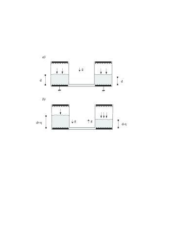
Figure 2: A system with $\Sigma<\Sigma_{0}$ when the pressure instability mechanism is possible ($\Sigma<\sqrt{\varepsilon_{l}}$). Long white arrows indicate the action of electrical pressure jump. In (b), when a perturbation is introduced, we see a gravitational force appear. This gravitational pressure flow, directed towards the cylinder with lower interface height in all cases, is $2\left<\rho\right>g\eta$ (or $2\xi$ in reduced magnitudes). In this case, the net electric pressure flow is directed towards the left cylinder (three arrows against one).

If a plane perturbation is introduced, the magnitude $\Sigma$ gets in general a value $\Sigma_{-}$ in the cylinder with a minimum interface elevation and another value $\Sigma_{+}$ in the cylinder with maximum elevation. But in order to simplify, let us restrict to an infinitesimal perturbation, so the new values still fulfill $\Sigma_{\pm}<\Sigma_{0},\varepsilon_{l}$. Once the perturbation is introduced, a gravitational pressure acts against it by communicating an upwards pressure to the zone with minimum interface elevation (figure 2b). Now the electric pressure jump (13) is higher in the zone with a lower interface height as the thickness of the lower fluid layer has decreased. Conversely, in the zone of maximum elevation the electric pressure jump decreases. Thus, a net electric pressure flow appears towards the left cylinder in figure 2(b). If the difference between the electrical pressure jump in both cylinders is high enough, the restoring action of the gravitational pressure will be counterbalanced. This is possible if the applied potential is higher than a critical value $V_{c}$, given by the stability condition (7).

On the contrary (figure 3a), if the electrical pressure jump magnitude still decreases with the lower layer thickness but becomes negative ($\sqrt{\varepsilon_{l}}<\Sigma<\Sigma_{0}$), the perturbation is damped (figure 3b). The same analysis may be carried out when $E_{l}(z_{s})$ increases with the layer thickness of fluid $l$ ($\Sigma>\Sigma_{0}$), so finally two linearly stable regions are found: $\sqrt{\varepsilon_{l}}<\Sigma<\Sigma_{0}$ and $\Sigma_{0}<\Sigma<\sqrt{\varepsilon_{l}}$. Thus, the apparition of linearly stable bands is related to the change in the tendency of the electric pressure with the lower layer thickness, which gives the limit $\Sigma_{0}$, and to the change of electric pressure jump, which gives the limit $\varepsilon_{l}$.

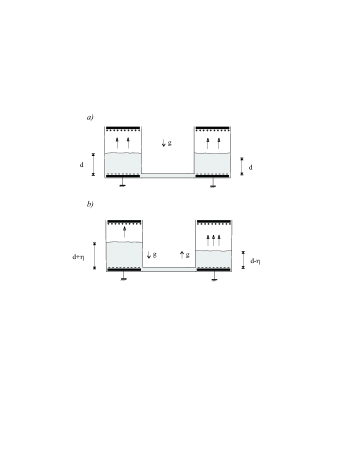
Figure 3: A system with $\Sigma<\Sigma_{0}$ when the pressure instability mechanism is not possible ($\Sigma>\sqrt{\varepsilon_{l}}$). We see now the net electric pressure flow is directed towards the right cylinder (lower interface height), in the same restoring direction that the restoring gravitational term: the electric pressure is stabilising.

We see that for a given behaviour of $E_{l}(z_{s})$, the stabilization is due to a change in the sign of the electric pressure jump. In order to find out what may cause this change of sign, let us write the electric pressure jump as a function of polarization ($Q_{p}=Q_{t}-Q$) and free interfacial charges. The contribution of the free surface charges to the electrical pressure jump has the same sign of the total interfacial charge term:

$$\left<\frac{1}{2}\varepsilon E^{2}\right>=\frac{1}{2}E_{l}(z_{s})\left[\frac{\Sigma}{\varepsilon_{0}}Q_{t}+Q\right]$$ (16)

while the contribution of the polarization charges has opposite sign to the term of total charge:

$$\left<\frac{1}{2}\varepsilon E^{2}\right>=\frac{1}{2}E_{l}(z_{s})\left[\left(1+\frac{\Sigma}{\varepsilon_{0}}\right)Q_{t}-Q_{p}\right]$$ (17)

Thus, we see that if no polarization charges are present initially, the electric pressure jump takes the sign of the total interfacial charge $Q_{t}$. If we now change $\varepsilon_{l}$ at constant $\Sigma$ in such a way that polarization charges have the same sign that $Q_{t}$ and get high enough, they can change the sign of the electric pressure jump. Thus, they play an essential role in the stabilization of the interface.

II.4 On the critical curves in the hydraulic model

It is also convenient to define the dimensionless parameter $U_{NL}=\varepsilon_{u}V_{c}^{2}/(\left<\rho\right>gd^{3})$ where $V_{c}$ is the applied potential for which the stability condition (7) is fulfilled (i.e., $V>V_{c}$ yields $\left<\Pi\right>_{-}-\left<\Pi\right>_{+}>0$ and the perturbation can be sustained). The parameter $U_{NL}$ represents the critical electric pressure $\varepsilon_{u}V_{c}^{2}/d^{2}$, reduced with the gravitational pressure $\left<\rho\right>gd$, while its square root $U_{NL}^{1/2}$ represents the reduced critical applied potential. $U_{NL}$ is in general a function of the perturbation amplitude $\xi$.

Let us start with an unperturbed state ($\xi=0$, $V^{2}<U_{NL}(\xi=0)$), where an arbitrary stationary perturbation with amplitude $\xi_{0}$ is introduced. Then a valid solution $U_{NL}(\xi_{0})$ from (15) should fulfill two conditions to make possible the perturbation be sustained:

i) $U_{NL}(\xi_{0})>0$.

ii) $V^{2}\geq U_{NL}(\xi_{0})$.

The first one comes from the definition of $U_{NL}$ because $U_{NL}(\xi_{0})<0$ should correspond to an imaginary critical potential. The second one is also necessary because $V^{2}\leq U_{NL}(\xi_{0})$ indicates that the perturbation is decreased to a lower value.

Typical critical curves $U_{NL}(\xi)$ are represented in figures 4(a) and 5. In these curves stable and unstable regions are delimited by the function $U_{NL}(\xi)$ and the behaviour of $U_{NL}(\xi)$ provides information about the evolution of the perturbation once it is introduced. An increasing $U_{NL}(\xi)$ in $\xi_{0}$ ($\partial U(\xi_{0})/\partial\xi>0$) means that the perturbation will not tend to increase for an applied potential $V=U_{NL}^{1/2}(\xi_{0})$, because for $\xi>\xi_{0}$, $V<U_{NL}^{1/2}(\xi)$ (the interface cannot overcome the restoring action of the gravitational pressure). And viceversa, a decreasing $U_{NL}$ in $\xi_{0}$ means that the perturbation will tend to increase if $V=U_{NL}^{1/2}(\xi_{0})$. The third case occurs when $\partial U(\xi_{0})/\partial\xi=0$. In this case, for $V=U_{NL}^{1/2}(\xi_{0})$ the perturbation will not increase if $\partial^{2}U_{NL}(\xi_{0})/\partial\xi^{2}>0$ but it will tend to increase if $\partial^{2}U_{NL}(\xi_{0})/\partial\xi^{2}<0$. In definitive, if $\partial U_{NL}(\xi_{0})/\partial\xi>0$ (or if $\partial U(\xi_{0})/\partial\xi=0$, $\partial^{2}U_{NL}(\xi_{0})/\partial\xi^{2}>0$) it may be said that ”stabilization” of the perturbation occurs at $V=U_{NL}^{1/2}(\xi_{0})$ and the point $\xi=\xi_{0}$ may be considered as a new point of stable interface position, that is different to the trivial solution $\xi=0$ of the initial equilibrium state. We call these points ”perturbed stable states” and as we will see they are only present in the non-ohmic/ohmic interface.

III Ohmic/ohmic interface

In the case of two ohmic fluids with conductivities $\sigma_{u}$, $\sigma_{l}$, we take $\sigma_{u}$ as unit for electric conductivity. Taking into account that in the stationary state $\nabla\cdot{\mathbf{j}}=0$, then $j_{u}=j_{l}=j$, $E_{u}=\sigma_{l}E_{l}$ and the expressions for the dimensionless stationary electric field and $\Sigma$ in the unperturbed state are the following:

$$E_{l}=V_{l}\quad\quad E_{u}=V_{u}/L=\sigma_{l}V_{l}/L\quad\quad\Sigma=\sigma_{l}$$ (18)

being $V_{l}$ and $V_{u}$ the electric potential drop through the lower and upper fluid layers inside the cylinders. As the perturbation is plane, the fields in the perturbed state are:

$$E_{l\pm}=\frac{V_{l\pm}}{1\pm\xi}\quad\quad E_{u\pm}=\frac{V_{u\pm}}{L\mp\xi}$$ (19)

where the upper signs stand for the magnitudes evaluated at $x=0$ and the lower signs stand for the magnitudes at $x=\lambda/2$.

Using $V=V_{u+}+V_{l+}=V_{u-}+V_{l-}$, we obtain:

$$\left<\frac{1}{2}\varepsilon E^{2}\right>_{\pm}=\frac{1}{2}\left(\varepsilon_{l}-\sigma_{l}^{2}\right)\frac{V_{l\pm}^{2}}{(1\pm\xi)^{2}}$$ (20)

$$V_{l\pm}=\frac{1\pm\xi}{\sigma_{l}\left(L\mp\xi\right)+\left(1\pm\xi\right)}V$$ (21)

In an ohmic/ohmic interface $\Sigma$ is a constant (18) and therefore we can make the interface at constant $\Sigma$ coincide with the real interface (constant conductivities of the fluids). It is also easy to find that $\Sigma_{0}=1$: $E_{l}(z_{s})$ always decreases with the $l$ layer thickness for $\Sigma<1$ and always increases for $\Sigma>1$ (19). Thus, given the conductivities and permittivities of the fluids, the interface should be stable respect to the pressure instability mechanism for any value of the electric field, if $\sqrt{\varepsilon_{l}}<\Sigma<1$ or $1<\Sigma<\sqrt{\varepsilon_{l}}$, following the analysis in §II.3. This can be confirmed by finding the function $U_{NL}$.

After some short calculations and using the stability condition in reduced magnitudes (15) we get $U_{NL}$ as a function of the perturbation amplitude and the other parameters of the system:

$$U_{NL}(\xi,\sigma_{l},\varepsilon_{l},L)=f(\sigma_{l},\varepsilon_{l},L){\mathcal{K}}(\xi,\sigma_{l},L)$$ (22)

where $f(\sigma_{l},\varepsilon_{l},L)$ and ${\mathcal{K}}(\xi,\sigma_{l},L)$ (which gives all the dependence on the perturbation amplitude $\xi$) are the following functions:

$$f(\sigma_{l},\varepsilon_{l},L)=\frac{1}{(\varepsilon_{l}-\sigma_{l}^{2})(1-\sigma_{l})(1+L\sigma_{l})}$$

$${\mathcal{K}}(\xi,\sigma_{l},L)=\left((1+L\sigma_{l})^{2}-(1-\sigma_{l})^{2}\xi^{2}\right)^{2}$$ (23)

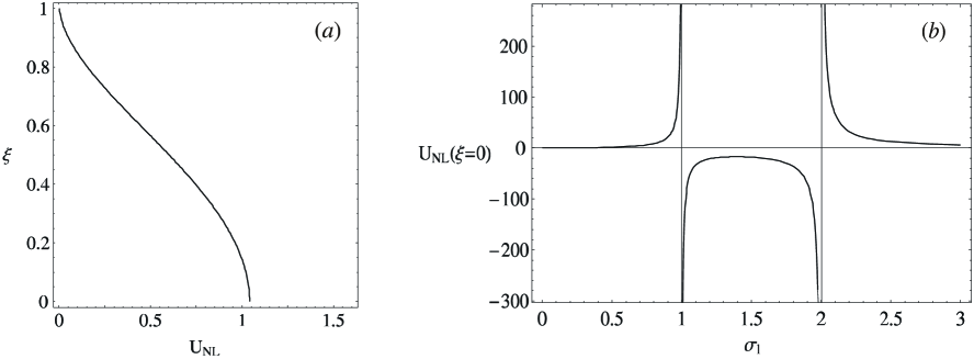
Figure 4: (a) The parameter $U_{NL}$ (if positive) is always decreasing with the perturbation amplitude; $\sigma_{l}=100$, $\varepsilon_{l}=4$, $L=1$. (b) The linear criterion ($U_{NL}(\xi=0)$) plotted against $\sigma_{l}$ presents a stable region (the negative values of $U_{NL}$), as a consequence of the action of polarization charges; $\varepsilon_{l}=4$, $L=1$.

It is to be noticed that for $\Sigma=\sigma_{l}=1$ and $\Sigma=\sigma_{l}=\sqrt{\varepsilon_{l}}$ the parameter $U_{NL}$ takes an infinite value for any $\xi$ (i.e., the instability is not possible), which is in accordance with the analysis in §II.3 ($\sigma_{l}=\sqrt{\varepsilon_{l}}$ is equivalent to $\Sigma=\sqrt{\varepsilon_{l}}$ and $\sigma_{l}=1$ gives $\left<\varepsilon E^{2}\right>_{-}=\left<\varepsilon E^{2}\right>_{+}$).

In an ohmic/ohmic interface, condition i) in §II.4 is fulfilled if and only if $f(\sigma_{l},\varepsilon_{l},L)>0$. This is so because the function ${\mathcal{K}}(\xi,\sigma_{l},L)$ is always positive (23). And the sign of $f(\sigma_{l},\varepsilon_{l},L)$ is positive (23) unless the terms ($1-\sigma_{l}^{2}/\varepsilon_{l}$) and ($1-\sigma_{l}$) have different signs. This occurs when $\sqrt{\varepsilon_{l}}<\sigma_{l}<1$ or $1<\sigma_{l}<\sqrt{\varepsilon_{l}}$; i.e., no perturbation can be sustained if the electrical pressure jump and the total surface charge $Q_{t}$ at the interface have opposite signs (see (14), (18), (20)). Thus, the result advanced by the analysis in §II.3 is confirmed by the explicit calculation of $U_{NL}$. Analysing further the conditions for stabilization we notice that they are fulfilled when the interfacial free charge $Q=(\varepsilon_{l}-\Sigma)E_{l}(z_{s})$ takes opposite sign to the total interfacial charge $Q_{t}$, and consequently the polarization charge $Q_{p}=Q_{t}-Q$ takes the sign of $Q_{t}$, which agrees again with the analysis performed in §II.3. Although the problem of the stability of an ohmic/ohmic interface has been extensively studied, this stabilizing effect due to polarization charges has not been formerly detected. The values of $U_{NL}$ are plotted in figure 4(b) vs. the reduced conductivity $\sigma_{l}$. The stable region corresponds to the interval where $U_{NL}$ takes negative values.

Besides, we saw in §II.4 too that for $V^{2}=U_{NL}(\xi_{0})$ the perturbation amplitude tends to grow up to $\xi_{1}>\xi_{0}$ from its initial value $\xi_{0}$ if $V^{2}\geq U_{NL}(\xi)$ inside the interval $(\xi_{1},\xi_{0})$, which is always the case in an ohmic/ohmic interface if conditions i) and ii) are fulfilled. In effect, let us study the derivative $\partial U_{NL}/\partial\xi$:

$$\frac{\partial U_{NL}}{\partial\xi}=f(\sigma_{l},\varepsilon_{l},L)\frac{\partial{\mathcal{K}}(\xi,\sigma_{l},L)}{\partial\xi}$$ (24)

$$\frac{\partial{\mathcal{K}}(\xi)}{\partial\xi}=-4\xi(\sigma_{l}-1)^{2}\left((1+L\sigma_{l})^{2}-(\sigma_{l}-1)^{2}\xi^{2}\right)$$

As we see, if $f(\sigma_{l},\varepsilon_{l},L)>0$, $\partial U_{NL}/\partial\xi$ is always negative (figure 4a), provided that $\xi<L$ (a perturbation with $\xi>L$ forces the interface to touch the upper electrode, case that we do not analyse). The result is independent of the initial of the values of $\xi_{0}$ and $\xi_{1}$. This means that in an ohmic/ohmic fluid interface the pressure mechanism is always self-fed as it becomes increasingly stronger: once the instability is set on the perturbation amplitude grows up to its maximum value. This is a well known characteristic of EHD instabilities in plane interfaces in ohmic systems de Surgy (1995).

For $\sigma_{l}\to\infty$, it is easy to find from (22) and (23) that $U_{NL}(\xi=0)=L^{3}$, wich agrees with the result by Taylor and McEwan (1965). And finally, the author has checked that for the linear instability at finite conductivities the critical values provided by the hydraulic model ($U_{NL}(\xi=0)$) coincide exactly with those of the complete linear theory for an infinite plane interface Melcher and Jr. (1969) in the case of an infinite wavelength instability with negligible charge relaxation effects, confirming the demonstration in §II.2.

We see then that although the instability in an infinite ohmic/ohmic interface has been extensively studied, the hydraulic model is able to reproduce some former basic results Melcher and Jr. (1969); de Surgy (1995) and also to find a new feature: the stabilizing effect of the polarization interfacial charges when combined with the action of free interfacial charges. But the most relevant new results of the hydraulic model are found in the non-ohmic/ohmic interface under unipolar injection, in the next section.

IV Non-ohmic/ohmic interface

IV.1 Equations

Let us suppose now that the fluid ”u” is in non-ohmic regime of electric conduction and the fluid ”l” is in ohmic regime. If there is a unipolar space charge source in the upper electrode, a unipolar space charge distribution is induced in the non-ohmic fluid, in which the conduction (in dimensional magnitudes) is expressed by ${\mathbf{j}_{u}}=q_{u}(K_{u}{\mathbf{E}}_{u}+{\mathbf{v}})-D\nabla q_{u}$; where $K_{u}$ is the ion mobility of non-ohmic fluid and $D_{u}$ its diffusion coefficient. The diffusion term may usually be neglected Atten and Moreau (1972), so in a state at rest (${\mathbf{v}}={\mathbf{0}}$) we have in our system that $j_{u}=K_{u}q_{u}E_{u}$ in the non-ohmic fluid. We take now $K_{u}\sqrt{\varepsilon_{u}\left<\rho\right>g/d}$ as unit for electric conductivity, being $K_{u}$ the ion mobility in fluid u. In reduced magnitudes we have the following electric equations in stationary regime (for which $\nabla\cdot{\mathbf{j}}=0$):

$$j_{u}=q_{u}E_{u}=j\quad\quad\frac{dE_{u}}{dz}=q_{u}$$ (25)

$$j_{l}=\sigma_{l}E_{l}=j\quad\quad\frac{dE_{l}}{dz}=0$$ (26)

with the boundary conditions in the electrodes:

$$\phi_{u}(-L)=1\quad\quad q_{u}(-L)=C\quad\quad\phi_{l}(1)=0$$ (27)

and in the interface:

$$\phi_{u}(0)=\phi_{l}(0)\quad\quad j_{u}(0)=j_{l}(0)=j$$ (28)

where the condition $q_{u}(-L)=C$ denotes the fact that there is a space charge source at $z=-L$. The parameter $C$ represents the reduced space charge that the upper electrode injects on and is usually called ”level of injection”. The non-ohmic conduction due to unipolar injection and the correct boundary condition for a unipolar injection source $q_{u}(-L)$ have been studied in detail by Atten (Atten and Moreau, 1972; Lacroix, Atten, and Hopfinger, 1975, and references therein for more details on this issue).

Then the solution of the stationary electric field is:

$$E_{u}(z)=\sqrt{2j(z+b)}\quad\quad E_{l}(z)=\frac{j}{\sigma_{l}}\quad\quad\Sigma=\sqrt{\frac{2b}{j}}\sigma_{l}$$ (29)

with $b=\frac{j}{2C^{2}}+L$.

We see that now $\Sigma$ is not a constant but a function of the electric field (through the current density) and it is always possible for any real interface (i.e., any given value of $\sigma_{l}$) in the initially unperturbed state to find ranges of the electric field for which its corresponding $\Sigma$ lies out of the stable intervals: there exist real $U_{NL}(\xi=0)$ which are solution of the stability condition (7) for all values of $\sigma_{l}$. This means that the linearly stable region around the intervals $\sqrt{\varepsilon_{l}}<\Sigma<\Sigma_{0}$ or $\Sigma_{0}<\Sigma<\sqrt{\varepsilon_{l}}$ only exist as a consequence of dimensionalization and therefore they should disappear for a real interface (constant $\sigma_{l}$). In any case we will see in §IV.4 that now the action of polarization charges affects the pressure instability mechanism in other ways.

If the system is under strong injection conditions (i.e., $C\to\infty$), the expressions for the electric field and $\Sigma$ in the unperturbed interface are the following:

$$E_{l}(0)=V_{l}\quad\quad E_{u}(0)=\sqrt{2jL}=\sqrt{2\sigma_{l}V_{l}L}\quad\quad\Sigma=\sqrt{\frac{2\sigma_{l}L}{V_{l}}}$$ (30)

If a plane perturbation of amplitude $\xi$ is introduced, the equation for the electric pressure jump in the cylinder at the interface is:

$$\left<\frac{1}{2}\varepsilon E^{2}\right>_{\pm}=\frac{1}{2}\left[\varepsilon_{l}\frac{V_{l\pm}^{2}}{(1\pm\xi)^{2}}-2V_{l\pm}\sigma_{l}\left(\frac{L\mp\xi}{1\pm\xi}\right)\right]$$ (31)

The electric pressure jump can be expressed as a function of the applied potential $V$ taking into account: $j_{u+}=j_{l+}$, $j_{u-}=j_{l-}$ and $V=V_{u-}+V_{l-}=V_{u+}+V_{l+}$ for the electric potential. Then, in the perturbed interface we get:

$$(V-V_{l\pm})^{2}=\beta_{\pm}V_{l\pm}$$ (32)

where $\beta_{\pm}=\sigma_{l}(L\mp\xi)^{3}/(1\pm\xi)$.

From (32), we get the solution of $V_{l\pm}$:

$$V_{l\pm}=\frac{1}{2}\left(2V+\beta_{\pm}-\sqrt{\beta_{\pm}^{2}+4\beta_{\pm}V}\right)$$ (33)

The other root of (32), the one corresponding to the sign $+$ before the square root, is not possible as it gives a solution of $V_{l\pm}$ such that $V_{l\pm}>V$. In effect, as $\sqrt{\beta^{2}+4\beta V}>\beta$:

$$V_{l\pm}=\frac{2V+\beta_{\pm}+\sqrt{\beta_{\pm}^{2}+4\beta_{\pm}V}}{2}>\frac{2V+\beta_{\pm}}{2}>V$$ (34)

The value of $\Sigma_{0}$ is not constant in the non-ohmic/ohmic interface (from (31) and (33)) and in general $\Sigma_{0}\neq 1$, unlike in the ohmic/ohmic case. We introduce the expressions for the electric pressure jumps in the stability condition in reduced magnitudes (15) and then we get:

$$\left(\varepsilon_{l}\frac{V_{l-}^{2}}{(1-\xi)^{2}}-2\sigma_{l}V_{l-}\frac{L+\xi}{(1-\xi)}\right)-\left(\varepsilon_{l}\frac{V_{l+}^{2}}{(1+\xi)^{2}}-2\sigma_{l}V_{l+}\frac{L-\xi}{(1+\xi)}\right)=4\xi$$ (35)

As $V_{l+}$ and $V_{l-}$ are, from (33), determined by $V$, when the equality is held in (35) we get the condition of minimum applied potential $U_{NL}^{1/2}$ for which the instability mechanism is possible. Unlike in the ohmic/ohmic case, now (in general) there is no analytical expression for $U_{NL}$.

IV.2 Perfect conductor limit

Let us suppose that the ohmic fluid is a perfect electric conductor ($\sigma_{l}\to\infty$). In this limit $V_{l}\to 0$ and then:

$$\left<\frac{1}{2}\varepsilon E^{2}\right>_{\pm}\to\frac{1}{2}E_{u\pm}^{2}~{}\propto~{}\sigma_{l}V_{l\pm}=\frac{\sigma_{l}}{2}\left(2V+\sigma_{l}a_{\pm}-\sigma_{l}a_{\pm}\sqrt{1+\frac{4V}{\sigma_{l}a_{\pm}}}\right)$$ (36)

where $a_{\pm}=(8/9)(L\mp\xi)^{3}/(1\pm\xi)$.

We analyse the limit of $\sigma_{l}V_{l}$ when $\sigma_{l}\to\infty$. Developing the square root in power series of $1/\sigma_{l}<<1$, we get from (35) and (36):

$$U_{NL}=\frac{4}{9}\mathcal{F}(\xi)$$ (37)

being $\mathcal{F}(\xi)$:

$${\mathcal{F}}(\xi)=\frac{4\xi(L^{2}-\xi^{2})^{2}}{(L+\xi)^{2}-(L-\xi)^{2}}=\frac{1}{L}\left(L^{2}-\xi^{2}\right)^{2}$$ (38)

The function $\mathcal{F}(\xi)$ gives the variation of the non-linear criterion with the perturbation amplitude $\xi$.

Let us compare now with the case without charge injection ($C=0$). In the absence of injection the solution of the electric field at the interface tends to $E_{u\pm}\to V_{u\pm}/(L\mp\xi)$. Operating in a similar way to the strong injection case we have:

$$U_{NL}=\mathcal{F}(\xi)$$ (39)

that is exactly the same to the case of strong injection (37) except for the factor $4/9$ that now does not appear.

The dependence of $U_{NL}$ (and $U_{NL}^{1/2}$) with $\xi$ is, from (37, 39), the same for $C=\infty$ and $C=0$ and is given by the function $\mathcal{F}(\xi)$ (or $\mathcal{F}^{1/2}(\xi)$ for $U_{NL}^{1/2}$). We can see this behaviour of $U_{NL}^{1/2}(\xi)$ in fig. 5(a): for $\sigma_{l}=\infty$ (and hence, also for $\sigma_{l}=0$), $U^{1/2}_{NL}$ is always a decreasing function of $\xi$. Then, once the instability starts it tends abruptly to states with a minimum $U_{NL}$, which are the ones having a maximum value of the perturbation amplitude. An analogous behaviour has been experimentally observed in a conducting liquid with Koulova-Nenova et al. (1996) and without injection Taylor and McEwan (1965); de Surgy (1995), who observed that the instability develops violently towards the upper electrode, producing an electric breakage.

In the limit of zero perturbation amplitude the linear criterion for the instability in a perfect conducting fluid interface can be reobtained. In effect, if ${\xi\to 0}$ we obtain that ${\mathcal{F}}(\xi)\to L^{3}$, and then $U_{NL}^{1/2}=L^{3/2}$ for the case without injection, which agrees with previous works Taylor and McEwan (1965); de Surgy (1995) and $U_{NL}^{1/2}=(2/3)L^{3/2}$ for the case with infinite injection, which agrees again with the result in former works Atten and Koulova-Nenova (1999); Vega and Pérez (2002a). Note also that the case $C=0$ yields the same criterion that in the ohmic/ohmic case for $\sigma_{l}\to\infty$, in §III.

IV.3 Non-conductor limit

Analogously, the non-conductor limit can be taken. Developing (35) in power series of $\sigma_{l}\ll 1$, and in the limit of $\sigma_{l}\to 0$ we get:

$$U_{NL}=\left(\frac{1}{\varepsilon_{l}}\right)\frac{4\xi(1-\xi^{2})^{2}}{(1+\xi)^{2}-(1-\xi)^{2}}=\frac{1}{\varepsilon_{l}}\left(1-\xi^{2}\right)^{2}=\frac{1}{\varepsilon_{l}}{\mathcal{H}}(\xi)$$ (40)

where now before the function of $\xi$ appears a factor $1/\varepsilon_{l}$ instead of the 4/9 in the perfect conductor. The value $\sigma_{l}=0$ has not real physical meaning but it is interesting the study of this limit as a reference for very low conductivities. In definitive, the behaviour of $U_{NL}^{1/2}(\xi)$ for $\sigma_{l}\ll 1$ is similar to that in the limit $\sigma_{l}\to\infty$, represented in figure 5(a). This can be seen analytically in the function ${\mathcal{H}}(\xi)$, which has the same behaviour that the function ${\mathcal{F}}(\xi)$: $U_{NL}(\xi)$ is always decreasing and is zero for the maximum perturbation amplitude. A similar behaviour is detected in experiments in very low conducting liquids under unipolar injection: the rose-window instability has a high deformation amplitude (of the order of the liquid layer thickness) near the instability threshold Vega (2002). The peculiarity respect to the high conducting case is that now the electric pressure is directed downwards.

The zero perturbation amplitude limit, $\xi\to 0$, yields ${\mathcal{H}}(\xi)=1$ and $U_{NL}^{1/2}=1/\sqrt{\varepsilon_{l}}$, which agrees with the result in the linear theory for the infinite interface Vega and Pérez (2002a).

IV.4 Non-linear transition from conducting regime to low conducting regime

In §IV.2 and §IV.3, we have demonstrated that in the limits of a non-conductor and perfect conductor ohmic layer $U_{NL}(\xi)$ is minimum for the maximum perturbation amplitude. This means that the instability, once is set on, evolves up to the maximum perturbation amplitude. The difference between both limits comes from the fact that while in the perfect conductor the instability is due to an upward electric pressure, in the non-conductor limit the instability is driven by a downward electric pressure. It seems reasonable to think that between the perfect conductor and the non-conductor behaviour there should be intermediate behaviours, i.e., perturbations that do not grow up to the maximum value. In effect, we saw in §IV.1 that the real non-ohmic/ohmic interface is always initially unstable: it is possible to find a finite value of the applied electric field that is able to sustain any finite perturbation, which is a consequence of the non-constancy of $\Sigma$ (30) in the non-ohmic/ohmic case. But this does not prevent, after the instability is set on, the interface from entering a stabilizing behaviour. There would be two possibilities: one is that the electric pressure jump changes sign, and the other is that this pressure jump changes its behaviour with the lower layer thickness, while the interface is evolving. Either of the two possibilities could make the interface enter the stable intervals $\Sigma_{0}>\Sigma>\sqrt{\varepsilon_{l}}$ and $\sqrt{\varepsilon_{l}}>\Sigma>\Sigma_{0}$. We recall this is possible in the non-ohmic/ohmic interface only because the apparent conductivity (30) is not constant, and thus the interface is taking new $\Sigma$ values as the perturbation evolves. Thus, although linear stable states do not exist now for any value of $\sigma_{l}$, it should be possible to think in these cases of an instability that evolves without reaching the maximum perturbation amplitude: we say that perturbed states are expected to appear.

We saw in §II.4 that the perturbed stable states occur in an interval of $\xi$ when $\partial U_{NL}/\partial\xi>0$ in it. And, in effect, critical points of this type are calculated for the first time in this work, in figure 5(b), where $U_{NL}^{1/2}$ is plotted for a non-dimensional conductivity $\sigma_{l}=10^{4}$. This reduced conductivity corresponds in an air/liquid interface to a physical conductivity of the order of $10^{-2}~{}\Omega^{-1}$m^-1 when the dimension of the system is of about 1 cm. We see in figure 5(b)that the function $U_{NL}(\xi)$ (or, equivalently $U_{NL}(\xi)^{1/2}$) obtained from (35) has an increasing behaviour near the maximum amplitude. This means that a fluid much more conducting than water, for example, shows such stabilization, which could be possible even for an initial value $\xi_{0}=0$ and $V=U_{NL}^{1/2}(0$) as once the interface reaches the increasing $U_{NL}^{1/2}(\xi)$ region it begins to be decelerated as soon as it takes a value $\xi_{1}$ for which $V<U_{NL}^{1/2}(\xi_{1})$.

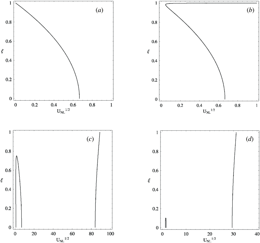
Figure 5: $U_{NL}^{1/2}$ as a function of the non-linear perturbation amplitude $\xi$ in a non-ohmic/ohmic interface under strong injection (dimensionless $L=1$, $\varepsilon_{l}=4$ in all figures). (a) For a non-ohmic/perfect conducting interface. (b) For a high non-dimensional conductivity value ($\sigma_{l}=10^{4}$). (c) For a lower non-dimensional conductivity ($\sigma_{l}=20$) three solutions in $\xi=0$ appear. (d) The two first solutions in $\xi=0$ tend to disappear if the conductivity is still lowered ($\sigma_{l}=7$).

We saw in the linear theory for an infinite plane interface that there may exist multiple instability threshold values for a given conductivity Vega and Pérez (2002a). This also occurs in the hydraulic model because if we further decrease the conductivity, three solutions at $\xi=0$ begin to appear (figure 5c). Two of them enclose an unstable region which should correspond with the high conducting regime-like instability (upward electric pressure jump) while the third one corresponds to the low conducting mechanism (downward electric pressure jump). The two solutions enclosing an unstable region get nearer as the conductivity is decreased (figure 5d): the conducting mechanism tends to disappear. Finally, for lower conductivities, a unique solution at $\xi=0$ corresponds to the non-conductor limit of (40). The value of $\Sigma$ (30) can be used to determine the corresponding pressure mechanism.

Figure 6 represents $U_{NL}^{1/2}($$\xi$$=0)$ as a function of the conductivity $\sigma_{l}$. The curves from the stability condition for the hydraulic model (7) show the same qualitative behaviour that the linear critical values from the stability condition for the infinite interface (12). In addition, the linear critical values from (12) coincide (figure 6) with those for an infinite interface in the dimensional representation (scaled to our dimensionless magnitudes) of a previous work Vega and Pérez (2002a), which confirms that the stability condition (12) applies for an infinite interface. The quantitative similarity of the results from (7) and (12) in figure 6 suggests also that additional term in the stability condition for the infinite interface is less important. Thus, the limits of the stable bands detected in the dimensionless representation of the author’s previous work Vega and Pérez (2002a) must be close the limit values for the hydraulic model: $\sqrt{\varepsilon_{l}}$ and $\Sigma_{0}$. Thus, the stable bands are related to the change of electric pressure jump sign and the change of tendency of the electric pressure jump with layers relative thickness, instead of being related to the change of sign in the interfacial charge, as suggested previously Vega and Pérez (2002a) (notice, too, that the change of sign of interfacial charge does not provide two limits but just one value).

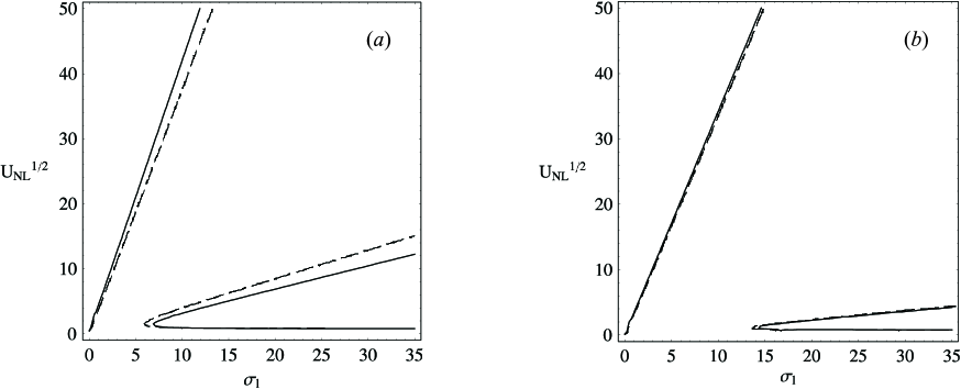
Figure 6: Reduced critical potential $U_{NL}$ vs. reduced conductivity $\sigma_{l}$ for an infinitesimal perturbation $\xi\to 0$ with $L=1$. Continuous curve stands for the hydraulic model stability condition (7) while discontinuous curve stands for both the stability condition in a previous work and (12). (a) Reduced dielectric constant $\varepsilon_{l}=4$. (b) Reduced dielectric constant $\varepsilon_{l}=40$. The effect of increasing the dielectric constant (i.e., increasing the polarization interfacial charges in the high conducting region) in the non-ohmic/ohmic interface is to move the conducting critical curve (the one at the right) to higher values of $\sigma_{l}$.

V Conclusions

We study a hydraulic model, for which we find a non-linear stability condition, with a twofold objective:

First, to study specifically the unstabilizing mechanism of electric pressure jump against the gravitational force, we use a dimensionless representation in which we introduce the fundamental parameter ”apparent conductivity” ($\Sigma$). This allows a systematic study of the different types of electric pressure unstabilising mechanisms. The simple and intuitive hydraulic model and the use of the apparent conductivity, allow us to find two stability bands and their origins. This is in the action of polarization charges, that may inhibit the instability pressure mechanism in an interface subjected to a vertical field when combined to free interfacial charges. In our formulation, the stability bands are: $\Sigma_{0}>\Sigma>\sqrt{\varepsilon_{l}}$ and $\sqrt{\varepsilon_{l}}>\Sigma>\Sigma_{0}$, where $\varepsilon_{l}$ and $\Sigma_{0}$ are the reduced dielectric constant and the value of the apparent conductivity for which the electric pressure passes from decreasing to increasing with the reduced lower layer thickness. As a consequence of this, the pressure instability mechanism is not possible for any ohmic/ohmic interface with reduced conductivity $\sigma_{l}$ in the intervals $1>\sigma_{l}>\sqrt{\varepsilon_{l}}$ and $\sqrt{\varepsilon_{l}}>\sigma_{l}>1$; i.e., the total surface charge and the electric pressure jump at the interface have opposite signs. In the case of a non-ohmic/ohmic interface, the pressure instability mechanism is always possible, for any value of the ohmic conductivity, when we pass to the representation in $\sigma_{l}$.

In the hydraulic model there is also a transition region Vega and Pérez (2002a) in the pressure instability mechanism in a non-ohmic/ohmic interface for a linear perturbation, but also for a non-linear perturbation. The behaviour of the parameter $U_{NL}$ (or $U_{NL}^{1/2}$) as a function of the perturbation amplitude reveals the existence, for intermediate conductivities, of perturbed stable states (which are different to the trivial solution of the initial equilibrium state $\xi=0$). These new stable states are only found in the non-ohmic/ohmic interface, suggesting the possibility of interfacial dynamics very different to those detected in systems without injection Taylor and McEwan (1965); Melcher (1963); Melcher and Jr. (1969). This could be related to the observations by de Surgy (1995) of stabilised metallic points. In the limits of very low or high conductivity the behaviour of the function $U_{NL}^{1/2}(\xi)$ is as expected (analogous to the observed in the infinite interface): the instability evolves up to the maximum value of perturbation amplitude.

Although a detailed study of the interfacial dynamics is needed in order to do determine precisely the situations in which the stabilisation in perturbed states from any initial state is possible, it seems evident that the introduction of the injection enriches the behaviour of the pressure equilibria in a fluid interface, and also opens a way to stabilization and control of the interface deformation of high conducting fluid interfaces by applying stationary electric fields.

The second main objective of this work is to approach, in a mathematically simple way, the stability condition found in a previous work for an infinite non-ohmic/ohmic interface under unipolar injection, in the limit of long wavelength Vega and Pérez (2002a). In this issue, an equivalent stability condition to the referred one is found in a very simple way, in §II.2. The difference between the linear stability conditions in the hydraulic model (7) and in the infinite interface (12) was also found. This allows us to determine if there are cases in which these conditions coincide. We found that this coincidence occurs in the case of an ohmic/ohmic interface and also in the non-ohmic/ohmic interface in the limits of perfect conducting and very low conducting ohmic fluid. We also found that for intermediate conductivities, the difference between linear critical values given by the two stability conditions (7, 12) is not important (figure 6). This allows us to assert that the limits of the stability bands found are actually related to the values $\sqrt{\varepsilon_{l}}$ and $\Sigma_{0}$ and not to the interfacial total charge change of sign, like stated in the former author’s work Vega and Pérez (2002a).

It is interesting to stress that the hydraulic model has the added value of being simple and intuitive. This has allowed us to find, for the first time, the stabilizing behaviour of polarization charges in the ohmic/ohmic interface, even though this type of interface has been extensively studied (this result is also valid for the infinite interface). In the non-omhic/ohmic interface, the model also allowed us to find out the true reason for the appearance of stability bands in the non-dimensional formulation in a previous work Vega and Pérez (2002a). Thus, the hydraulic model allows us to find new unknown features and to correct mistaken interpretations in previously studied systems. The hydraulic model also sets a reference frame that can be used to find out for what values of the system parameters (conductivities, ion mobilities, dielectric constants, relative thicknesses, etc.) the electric pressure is acting as a destabilising mechanism in a two layer fluid interface. In addition, the model and its relation to the standard problem of a long wave perturbation in an infinite interface, has been set in a very formal and general approach. This allows for the model to be used as a first step to study a variety of interfacial (linear and non-linear) stability problems.