Non-linear amplification of small spin precession using long range dipolar interactions

Abstract

In measurements of small signals using spin precession the precession angle usually grows linearly in time. We show that a dynamic instability caused by spin interactions can lead to an exponentially growing spin precession angle, amplifying small signals and raising them above the noise level of a detection system. We demonstrate amplification by a factor of greater than 8 of a spin precession signal due to a small magnetic field gradient in a spherical cell filled with hyperpolarized liquid ¹²⁹Xe. This technique can improve the sensitivity in many measurements that are limited by the noise of the detection system, rather then the fundamental spin-projection noise.

Observation of spin precession signals forms the basis of such prevalent experimental techniques as NMR and EPR. It is also used in searches for physics beyond the Standard Model Regan ; Bear ; RomalisEDM ; Hunter96 and sensitive magnetometery Kominis . Hence, there is significant interest in the development of general techniques for increasing the sensitivity of spin precession measurements. Several methods for reducing spin-projection noise using quantum non-demolition measurements have been explored Bigelow ; Mabuchi and it has been shown that in some cases they can lead to improvements in sensitivity Budker ; Lukin . In this Letter we demonstrate a different technique that increases the sensitivity by amplifying the spin precession signal rather than reducing the noise.

The amplification technique is based on the exponential growth of the spin precession angle in systems with a dynamic instability caused by collective spin interactions. Such instabilities can be caused by a variety of interactions, for example, magnetic dipolar fields in a nuclear-spin-polarized liquid Warren ; Jeener99 ; Sauer or electron-spin polarized gas Vasilyev , spin-exchange collisions in an alkali-metal vapor Klipstein or mixtures of alkali-metal and noble-gas atoms Kornack . This amplification technique can be used in a search for a permanent electric dipole moment in liquid ¹²⁹Xe Romalis2001 . It is also likely to find applications in a variety of other systems with strong dipolar interactions, such as cold atomic gases Pfau and polar molecules Demille .

Consider first an ensemble of non-interacting spins with a gyromagnetic ratio $\gamma$ initially polarized in the $\hat{x}$ direction and precessing in a small magnetic field $B_{z}$. The spin precession signal $\langle S_{y}\rangle=\gamma\langle S_{x}\rangle B_{z}t$ grows linearly in time for $\gamma B_{z}t\ll 1$. The measurement time $t_{m}$ is usually limited by spin relaxation processes and determines, together with the precision of spin measurements $\delta(\langle S_{y}\rangle)$, the sensitivity to the magnetic field $B_{z}$

$$\delta B_{z}=\frac{\delta(\langle S_{y}\rangle)}{\gamma\langle S_{x}\rangle t_{m}}$$ (1)

or any other interaction coupling to the spins. In the presence of a dynamic instability, the initial spin precession away from a point of unstable equilibrium can be generally written as $\langle S_{y}\rangle=\gamma\langle S_{x}\rangle B_{z}\sinh(\beta t)/\beta$, where $\beta$ is a growth rate characterizing the strength of spin interactions. The measurement uncertainty is now given by

$$\delta B_{z}=\frac{\delta(\langle S_{y}\rangle)\beta}{\gamma\langle S_{x}\rangle\sinh(\beta t_{m})}.$$ (2)

Hence, for the same uncertainty in the measurement of $\langle S_{y}\rangle$, the sensitivity to $B_{z}$ is improved by a factor of $G=\sinh(\beta t_{m})/\beta t_{m}$. It will be shown that quantum (as well as non-quantum) fluctuations of $\langle S_{y}\rangle$ are also amplified, so this technique cannot be used to increase the sensitivity in measurements limited by the spin-projection noise. However, the majority of experiments are not limited by quantum fluctuations. For a small number of spins the detector sensitivity is usually insufficient to measure the spin-projection noise of $N^{1/2}$ spins, while for a large number of particles the dynamic range of the measurement system is often insufficient to measure a signal with a fractional uncertainty of $N^{-1/2}$. Amplifying the spin-precession signal before detection reduces the requirements for both the sensitivity and the dynamic range of the measurement system. Optical methods allow efficient detection of electron spins and some nuclear spins RomalisEDM in atoms or molecules with convenient optical transitions. However, for the majority of nuclei optical detection methods are not practical and magnetic detection, using, for example, magnetic resonance force microscopy, has not yet reached the sensitivity where it is limited by the spin projection noise Sidles ; Thurber . Therefore, non-linear amplification can lead to particularly large improvements in precision measurements relying on nuclear spin precession.

Here we use long-range magnetic dipolar interactions between nuclear spins that lead to exponential amplification of spin precession due to a magnetic field gradient Jeener99 ; Romalis2001 ; Ledbetter2002 . It has also been shown that long-range dipolar fields in conjunction with radiation damping due to coupling with an NMR coil lead to an increased sensitivity to initial conditions and chaos Lin . To amplify a small spin precession signal above detector noise it is important that the dynamic instability involves only spin interactions, since instabilities caused by the feedback from the detection system would couple the detector noise, such as the Johnson noise of the NMR coil, back to the spins. We measure spin precession using SQUID magnetometers that do not have a significant back-reaction on the spins and show that under well controlled experimental conditions the dynamic instability due to collective spin interactions can be used to amplify small spin precession signals in a predictable way.

Our measurements are performed in a spherical cell containing hyperpolarized liquid ¹²⁹Xe (Fig. 1). Liquid ¹²⁹Xe has a remarkably long spin relaxation time Romalis2001 and the spin dynamics is dominated by the effects of long-range magnetic dipolar fields. In the spherical geometry an analytic solution can be found using a perturbation expansion in a nearly uniform magnetic field $H_{0}$ Romalis2001 ; Ledbetter2004 . We are primarily interested in the first-order longitudinal magnetic field gradient $g$, $\mathbf{H}=(H_{0}+gz)\mathbf{\hat{z}}$, but will also consider other magnetic field gradients which inevitably arise due to experimental imperfections. For longitudinal gradients that preserve cylindrical symmetry the magnetization profile can be expanded in a Taylor series,

$$\mathbf{M}(\mathbf{r},t)=\mathbf{M}_{0}+M_{0}\sum_{i,k}\mathbf{m}^{(i,k)}(t)\frac{z^{i}(x^{2}+y^{2})^{k}}{R^{i+2k}},$$ (3)

where $R$ is the radius of the cell. Only gradients of the magnetization create dipolar fields in a spherical cell, for example, a linear magnetization gradient $\mathbf{m}^{(1,0)}$ creates only a linear dipolar magnetic field, which, in the rotating frame, is given by

$$\mathbf{B}_{d}^{(1,0)}=\frac{8\pi M_{0}z}{15R}\left\{m_{x}^{(1,0)},m_{y}^{(1,0)},-2m_{z}^{(1,0)}\right\}.$$ (4)

The time evolution of the magnetization is determined by the Bloch equations $d\mathbf{M}/dt=\gamma\mathbf{M}\times(\mathbf{B}_{d}+\mathbf{H})$. If the magnetization is nearly uniform, $\mathbf{m}^{(i,k)}\ll 1$, they can be reduced to a system of linear first-order differential equations for $\mathbf{m}^{(i,k)}$.

Figure 1: Low field NMR setup (view from above). Polarized liquid ¹²⁹Xe is contained in a spherical cell maintained at 173K by flowing N₂ gas through a vacuum insulated column. High-$T_{c}$ SQUIDs are submerged in LN₂ contained in a glass dewar. Inset: configuration of the SQUIDs, applied magnetic field, the magnetization, and the rotatable membrane.

We consider first the simplest case when only the linear field gradient $g$ is present and the initial uniform magnetization $M_{0}$ is tipped into the $\hat{x}$ direction of the rotating frame by a $\pi/2$ pulse. Substituting Eqns. (3) and (4) into the Bloch equations we find that only linear magnetization gradients grow as long as $\mathbf{m}^{(i,k)}\ll 1$, in particular, $m_{y}^{(1,0)}$ is given by

$$m_{y}^{(1,0)}(t)=-\frac{\gamma gR}{\beta}\sinh(\beta t),$$ (5)

$$\beta=\frac{8\sqrt{2}\pi}{15}M_{0}\gamma.$$ (6)

Here $\beta$ is proportional to the strength of the long-range dipolar interactions. We measure $m_{y}^{(1,0)}$ experimentally by placing two SQUID detectors near the spherical cell as illustrated in Fig. 1 and measuring the phase difference $\Delta\phi$ between the NMR signals induced in the two SQUIDs. For small $m_{y}^{(1,0)}$, $\Delta\phi=\zeta m_{y}^{(1,0)}$, where $\zeta$ is a numerical factor that depends on the geometry, for our dimensions $\zeta=0.46\pm 0.01$. Thus, the phase difference $\Delta\phi$ is proportional to the applied magnetic field gradient $g$ and grows exponentially in time, increasing the sensitivity to $g$ by a factor $G=\sinh(\beta t)/\beta t$. For $M_{0}=100$ $\mu$G, which is easy to realize experimentally with hyperpolarized ¹²⁹Xe, $\beta=1.75~{}{\rm sec}^{-1}$, so that a very large amplification factor can be achieved in a short time, for example $G=360$ after 5 seconds.

One of the main challenges to realizing such high gains is to achieve sufficient control over the initial conditions and non-linear evolution of the system, so that the dynamic instability gives rise to a phase difference $\Delta\phi$ that remains proportional to $g$ even in the presence of various experimental imperfections. We developed a set of numerical and analytical methods for analyzing these effects Ledbetter2004 . Since our goal is to achieve very high sensitivity to a small first-order longitudinal magnetic field gradient $g$, we generally assume that it is smaller than other gradients that are not measured directly. We find that the presence of transverse or higher order longitudinal gradients as well as initial magnetization inhomogeneities cause an abrupt non-linear decay of the overall magnetization. The time until the decay $t_{c}$ depends on the size of the inhomogeneities relative to $M_{0}$ and limits the achievable gain to $\sinh(\beta t_{c})/\beta t_{c}$. Inhomogeneities of the applied field symmetric with respect to the $z$ direction do not change the evolution of $\Delta\phi$, which remains proportional to $g$ until the collapse of the magnetization, as shown in Fig. 2a. Higher order $z$-odd longitudinal gradients do generate a phase difference (Fig. 2b). However, the contributions of different magnetic field gradients to the phase difference add linearly as long as $\mathbf{m}^{(i,k)}\ll 1$ and the effects of higher order odd gradients can be subtracted if they remain constant, as illustrated in Fig. 2b. While higher order magnetization gradients can grow with a time constant up to 2.5 times faster than the first-order gradient, it can be shown using a perturbation expansion that the first moment of the magnetization $d=\int zM_{y}dV$ always grows with an exponential constant given by Eq. (6) and is proportional to the first moment of the magnetic field $b=\int zB_{z}dV$. The phase difference between the SQUID signals is approximately proportional to the first moment of the magnetization $d$ and is not significantly affected by the growth of higher order gradients. For example, in Fig. 2b) the overall signal decays at about 3 sec due to large first and third-order magnetization gradients but the phase difference $\Delta\phi$ remains much less than 1.

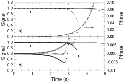
Figure 2: Numerical simulations Ledbetter2004 of the SQUID signal (left axis) and the phase difference between SQUIDs (right axis) for $M_{0}=100\thinspace\mu$G and a small longitudinal field gradient $g=0.1\thinspace\mu$G/cm (solid lines). a) An additional larger transverse gradient $g_{\perp}=2\thinspace\mu$G/cm (dashed line) or a second-order longitudinal gradient $g_{2}=1\thinspace\mu$G/cm² (dash-dot) do not affect the phase difference until the SQUID signal begins to decay. b) Effects of an additional $z$-odd third-order longitudinal gradient $g_{3}=0.8\thinspace\mu$G/cm³ (squares). Stars show the phase evolution in the presence of $g_{3}$ but for $g=0$. The difference between the phase for $g=0.1\thinspace\mu$G/cm and $g=0$ (triangles) follows the solid line corresponding to the pure linear gradient $g$ until the magnetization begins to collapse. The third-order gradient generates a background phase that can be subtracted to determine a change in $g$ between successive measurements.

Hence, the phase difference $\Delta\phi$ can be used to measure a very small linear gradient $g$ in the presence of larger inhomogeneities if all magnetic field and magnetization inhomogeneities are much smaller than $M_{0}$. The ultimate sensitivity is limited by fluctuations of the gradients between successive measurements. In addition to fluctuations of $g$, which is the quantity being measured, the phase difference will be affected by the fluctuations in the initial magnetization gradients $m_{y}^{(1,0)}$ and $m_{z}^{(1,0)}$ and, to a smaller degree, higher order $z$-odd gradients of the magnetic field and the magnetization. In particular, fluctuations of $m_{y}^{(1,0)}$ and $m_{z}^{(1,0)}$, either due to spin-projection noise or experimental imperfections, set a limit on the magnetic field gradient sensitivity on the order of $\delta g=8\pi\sqrt{2}M_{0}\delta m_{y}^{(1,0)}/15R$ and similar for $\delta m_{z}^{(1,0)}$. The shot noise fluctuations of ¹²⁹Xe magnetization generate a magnetic field gradient on the order of $10^{-13}$ G/cm.

Hyperpolarized ¹²⁹Xe is produced using the standard method of spin exchange optical pumping Romalis2001 ; Bastian . The polarized gas is condensed in a spherical glass cell held at 173 K as shown in Fig. 1. The cell, with an inner radius $R=0.55$ cm, is constructed from two concave hemispherical lenses glued together with UV curing cement. Inside the cell is an octagonal silicon membrane 25 $\mu$m thick, with a diameter of 1.05 cm. The membrane is connected to a stepper motor outside the magnetic shields via a  0.2 mm glass wire to mix the sample, ensuring uniformity of the polarization. In addition to mixing the sample, the membrane inhibits convection across the cell due to small temperature gradients which can wash out the longitudinal gradient of the magnetization. A set of coils inside the shields create a 10 mG uniform magnetic field and allow application of RF pulses and control of linear and quadratic magnetic field gradients. The NMR signal is detected using high-$T_{c}$ SQUID detectors. The pick-up coil of each SQUID detector is an 8$\times 8$ mm square loop located approximately 1.6 cm from the center of the cell and tilted by $\pm 45^{\circ}$ relative to the magnetic field.

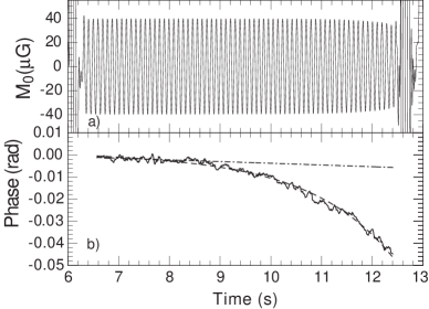
Figure 3: a) Oscillating transverse magnetization following a $\pi$/2 pulse. After the signal drops to 90% of its initial value a second pulse is applied to realign the magnetization with the longitudinal direction. b) Phase difference between the SQUID signals. Overlaying the data (dashed line) is a fit based on Eq. (5). The dash-dot line is the expected phase evolution in the non-interacting case, illustrating that the signal would barely be detectable.

In our experimental system, the time scale of the dipolar interactions is much smaller than the spin relaxation time or the time needed to polarize a fresh sample of ¹²⁹Xe. In order to make multiple measurements on a single sample of polarized xenon, we first apply a $\pi/2$ pulse and monitor in real time the SQUID signals. When the NMR signal drops to 90% of its initial value, a second $\pi/2$ pulse is applied, realigning the magnetization with the holding field. The silicon membrane is then oscillated back and forth to erase the magnetization inhomogeneities developed in the previous trial.

Fig. 3a) shows the oscillating transverse magnetization and Fig. 3b) shows the phase difference between the two SQUID signals. We determine the value of $\beta$ from the magnitude of the NMR signal and fit the phase difference to Eq. (5) with $g$ as the only free parameter. The dash-dot line shows the expected evolution of the phase difference for the same gradient in the absence of dipolar interactions, demonstrating that without amplification the phase difference would be barely above the noise level of the detection system. For this measurement the phase is amplified by a factor of 9.5 before the magnetization drops to 90% of its initial value.

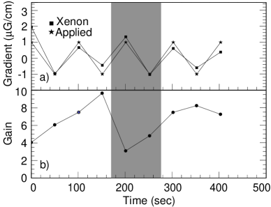
Figure 4: a) Measurement of a small gradient $g$ alternated between successive trials. Stars show the applied linear gradient, squares show the gradient measured using non-linear spin evolution. b) Gain $G$ associated with non-linear spin evolution. The gain drops when the sample is not mixed in the shaded region, demonstrating the significance of initial magnetization inhomogeneities.

By applying a series of double $\pi/2$ pulses we can make repeated measurements of the magnetic field gradient. Fig. 4a) shows data where the applied longitudinal gradient is oscillated with an amplitude of 1 $\mu$G/cm between trials. The stars show the applied gradient, the squares show the gradient measured by the non-linear spin evolution, indicating that the amplified signal follows the applied gradient. Slight differences between the two curves are due to noise in the magnetic field gradient as well as possible imperfections in the erasing of magnetization gradients between successive trials. Fig. 4b) shows the gain parameter for the same data set. We associate the rising gain at the beginning of the data set with a decay of the magnetization inhomogeneities developed during collection of liquid ¹²⁹Xe in the cell. In the shaded region of the plot we did not mix the magnetization with the membrane before the measurement, resulting in a drop of the gain as well. Numerical simulations indicate that the gain is likely limited by higher order gradients, for example a second-order magnetic field gradient on the order of 1 $\mu$G/cm², which can not be excluded based on our mapping of ambient fields, is sufficient to limit the gain to about 10.

In conclusion, we have demonstrated that non-linear dynamics arising from long range dipolar interactions can be used to amplify small spin precession signals, improving the signal-to-noise ratio under conditions where limitations of the spin detection system dominate the spin projection noise. By amplifying the signal before detection, this technique reduces the requirements on the sensitivity of the detection technique as well as its dynamic range. In addition to precision measurements, this technique can potentially be used to amplify small spin precession signals in various MRI applications, allowing, for example, direct detection and imaging of the magnetic fields generated by neurons with MRI Xiong . Initial inhomogeneities of the magnetization, caused, for example, by very slight differences of $T_{1}$ in tissues, can also be amplified. We thank DOE, NSF, the Packard Foundation and Princeton University for support of this project.

References

- (1) B.C. Regan, E.D Commins, C.J. Schmidt, and D. DeMille, Phys. Rev. Lett. 88, 071805 (2002).
- (2) D. Bear et al., Phys. Rev. Lett. 85, 5038 (2000).
- (3) M.V. Romalis, W.C. Griffith, J.P. Jacobs, and E.N. Fortson, Phys. Rev. Lett. 86, 2505 (2001).
- (4) A.N. Youdin et al., Phys. Rev. Lett. 77, 2170 (1996).
- (5) I.K. Kominis, T.W. Kornack, J.C. Allred, and M.V. Romalis, Nature 422, 596 (2003).
- (6) A. Kuzmich, L. Mandel, and N.P. Bigelow, Phys. Rev. Lett. 85 1594 (2000).
- (7) J.M. Geremia, J.K. Stockton and H. Mabuchi, Science 304, 270, (2004).
- (8) M. Auzinsh et. al, Phys. Rev. Lett. 93, 173002 (2004)
- (9) A. André, A. S. Sørensen, and M. D. Lukin, Phys. Rev. Lett. 92, 230801 (2004).
- (10) W.S. Warren et al., Science 281, 247 (1998).
- (11) J. Jeener, Phys. Rev. Lett. 82, 1772 (1999).
- (12) K. L. Sauer, F. Marion, P.-J. Nacher, and G. Tastevin, Phys. Rev. B 63,184427 (2001).
- (13) S. Vasilyev, J. Järvinen, A.I. Safonov, A.A. Kharitonov, I.I. Lukashevich, and S. Jaakkola, Phys. Rev. Lett. 89, 153002, (2002).
- (14) W.M. Klipstein, S. K. Lamoreaux, and E. N. Fortson Phys. Rev. Lett. 76, 2266 (1996).
- (15) T.W. Kornack and M.V. Romalis, Phys. Rev. Lett. 89, 253002 (2002).
- (16) M.V. Romalis and M.P. Ledbetter, Phys. Rev. Lett. 87, 067601 (2001).
- (17) S. Giovanazzi, A. Gorlitz, and T. Pfau, Phys. Rev. Lett. 89, 130401 (2002).
- (18) D. DeMille, Phys. Rev. Lett. 88, 067901 (2002).
- (19) J.A. Sidles et al., Rev. Mod. Phys. 67, 249 (1995).
- (20) K.R. Thurber, L.E. Harrel, and D.D. Smith, J.Mag.Res. 162, 336 (2003).
- (21) M.P. Ledbetter and M.V. Romalis, Phys. Rev. Lett. 89, 287601 (2002).
- (22) Y.Y. Lin, N. Lisitza, S.D Ahn, and W.S. Warren , Science 290, 118 (2000).
- (23) M.P. Ledbetter, I.M Savukov, L.-S. Bouchard, and M.V. Romalis , J. Chem. Phys. 121, 1454 (2004).
- (24) B. Driehuys et al., Appl. Phys. Lett. 69, 1668 (1996).
- (25) J.H. Xiong, P.T. Fox, and J.H. Gao, Hum. Brain Map. 20, 41 (2003).