Sub-collision hyperfine structure
of nonlinear-optical resonance
with field scanning

Abstract

Some experimental evidences for methane are produced that the simple transition from frequency scanning of nonlinear-optical resonances to magnetic one may be accompanied with transition from sub-Doppler collisionally broadened structure to sub-collision hyperfine one. It is conditioned by nonlinearity of splitting of hyperfine sublevel for molecules in the adiabatically varied magnetic field and respectively breaking the analogy of magnetic and frequency scannings. The exact calculation of the resonance structure is considered for molecules with only one spin subsystem. The approximately spin-additive calculation of the structure is given for sufficiently fast rotating molecules with greater number of spin subsystems. Within the same approximation an example of hyperfine doubling in the magnetic and electric spectra of nonlinear-optical resonance is considered for fluoromethane.

, , , and

1 Introduction

Nonlinear-optical resonance (NOR) is considered here in the intensity of laser radiation passed through molecular gas cell with low pressure ($\gtrsim 1\,\mathrm{mtorr}$). The laser frequency $\omega$ is tuned in a resonance with the frequency of spectral line $\omega_{mn}$, corresponding to investigated vibration-rotation transition ${[}^{m}_{n}$. The requirement to its fixing is practically absent and frequency detuning $\varOmega=\omega-\omega_{mn}$ can be somewhere in limits of Doppler width of this line.

The NOR (or NOR spectrum) can be scanned with laser frequency (NOR/Fr, i.e. NOR with frequency scanning). However we will take an interest in an alternative method of NOR scanning by means of varying external field while the laser frequency is invariable. It is supposed, that the resonancely absorbing gas is located in (spatially homogeneous and slowly varied) magnetic (/M) or electric (/E) field; the latter is meaningful to use only if there is a sublevel degeneration on parity. In both of the cases, there are two factors, namely, the crossings of field $M$-sublevels and the processes of their anti-crossings [in other words, processes of their repulsion, caused by hyperfine interactions in the initial (diagonalizing only field interactions) basis of wave functions] take place, respectively, with unequal and equal field projections $M$ of full angular momentum $F_{j}$ of a molecule in the hyperfine multiplets extracted by light, $(J_{j},I^{\bm{\cdot}})$ with $j=m,n$ [in the parentheses, respectively, rotation angular momentum of the molecule and spins of all its nuclei are designated] [2]. As a matter of fact and it will be shown in the given paper, just these two factors (and without collisional complexities) determine all major characteristics of a field spectrum of NOR. Let us underline the heterogeneity of the factors: the first is connected to diagonal elements of the interactions and the second to off-diagonal ones. Under transition in final (diagonalizing the sum of field and hyperfine interactions) wave function basis, the account of repulsing interactions of sublevels brings to that the amplitudes of hyperfine components of optical (electro-dipole) transition between these multiplets become field-dependent [3, Chap. 2 § 13]. Owing to the dependence, there are structures in field spectra of NOR, which we shall name “ballast” ones, underlining the energetic aspect of known process of anti-crossing of magnetic sublevels [4, 5]. With respect to Raman structures connected with crossings of magnetic sublevels, ballast ones have always opposite sign. They are present only in nonlinear-optical correction to a transmission of laser radiation and are absent in its birefringence. The ability of rotational (or, more precisely, vibration-rotational) subsystem to absorb a laser radiation will increase with hyperfine coupling of ballast spin subsystems. These ballast subsystems, if they are uncoupled, do not naturally interact with light themselves (from here the term “ballast”). Coupling (or uncoupling) implies a varying of hyperfine constants, however we reach that by the smooth varying of the external field, imposed on molecule gas, absorbing radiation. In this case, disbalancing of nuclear spin and rotation subsystems takes place, that can be effectively considered as a rupture of hyperfine couplings, see below (11). The disbalancing is possible because of usual distinction of Zeeman frequencies of a precession, i.e., when spin $g$-factor of any homogeneous nuclear subsystem of a molecule differs from rotation $g$-factor of the molecule. This preliminary qualitative picture will be verified in the following sections of our paper, and also we shall slightly touch upon linear Stark effect with its analogous electric spectra.

The NOR with field scanning (NOR/Fi, where option /Fi is /M or /E; one of advantages for given ranking of the letters consists in that the variable part of the abbreviation appears in the end) can be observed with various orientations of (amplitudely varied) external field $\bm{B}^{(0)}$ with respect to direction of wave vector $\bm{k}$ of laser radiation. The parallel or perpendicular orientation is used and respectively designated by subscript, $\parallel$ or $\perp$ after /Fi. The shape of NOR/Fi spectrum essentially depends from polarization of laser radiation.

From the very beginning of our research, the term “anomalous”, appearing below in description of an observed structure NOR/M_∥ for methane, implied its sub-collision property, i.e. a disposition inside collision contour of the resonance. It is necessary to take into account, that the constants of hyperfine interactions (HFI) in methane did not exceed its collision constant $\nu$ for our working pressure ($\gtrsim 1\,\mathrm{mtorr}$). The adequate theoretical model of NOR/M with this unusual property had find out only after the computer calculations, carried out for methane with the exact account of all its HFI.

NOR/Fr allows to look inside of inhomogeneous Doppler contour of a line. NOR/Fi, as we shall show below, allows to look inside of homogeneous collision contour of the same line, and we can observe a sub-collision hyperfine structure (HFS) [see below the respective equations (83), (85), and (89)].

Sometimes the field spectroscopy can be the real alternative to the frequency one. It is important, which type of field structures is selected. In the meantime it appears that the ballast HFS of NOR/Fi is more convenient and informative than Raman one. In this case the field spectroscopy can be viewed as a spectroscopy of intramolecular tops. We consider its variants for molecular levels without doubling and with doubling on parity. Respectively, our examples will be the molecules of methane and fluoromethane. For the first molecule all hyperfine (spin-rotation) constants can be spectrally determined, but for the second one they can be only partially determined from the spectra. Here to the aid there come researches of spin conversion in molecules [6, 7, 8]. These additional researches open a possibility of the determination of those hyperfine constants, which do not usually completely affect the spectra. The combined solution of these problems allows to receive the complete set of hyperfine spin-rotation constants for molecules of fluoromethane symmetry.

The purpose of this work is the theoretical research of influence hyperfine (spin-rotation) interactions on NOR/Fi in molecules of methane and fluoromethane symmetry. For it we are going:

• to analyze the probable reasons of appearance for “anomalous” structures of NOR/M in methane. It is necessary to make a choice between two models, one of theirs takes into account a HFS, other — a collision structure (it is exacter, a collision-hyperfine one).

• to apply the mathematical means that are adequate to the problem, i.e.  permitting to simplify the analysis of NOR/Fi caused by a multiplet structure of resonance levels.

• to receive an approximation (i.e. the first summands of expansion on a small parameter $J^{-2}$) for NOR/Fi in a case, when researched multispin molecule is in fast rotation states, and to apply the approximation to methane and fluoromethane. In the latter case we take into account hyperfine parity doubling for rotation $JK$-levels with $K=1$.

2 Some experimental evidences for a sub-collision structure
of NOR/M

When HFS of levels is absent or can be neglect, in a polarizing nonlinear sub-Dopppler spectroscopy there is a useful analogy between magnetic and frequency scanning of NOR. Let us begin from its brief description, see [9]. Let we have molecules in a gas cell and are capable optically to initiate electro-dipole transitions ${[}^{m}_{n}$ between two molecular vibration-rotation levels labelled with $j=m,n$ and degenerated on magnetic projections $M_{J_{j}}$ of rotation angular momentum with $J_{j}=\max(M_{J_{j}})$. We shall connect collision relaxation constants (level half-width $\nu_{j}$ and transition one $\nu$) by means of an equation $\nu_{m}+\nu_{n}=2\nu$; in all our examples it will completely be $\nu_{j}=\nu$. The gas cell is located in a varied magnetic field $\bm{B}^{(0)}=B^{(0)}\bm{u}_{z}$ and through it along the field a bichromatic light wave is propagated. Its electrical component

$$\bm{E}(r_{k},t)=\mathop{\mathrm{Re}}\sum_{q=\pm 1}E^{(\omega)}_{\underset{\scriptstyle\dot{}}{q}}(r_{k})\mathop{\mathrm{e}}\nolimits^{\mathrm{i}(kr_{k}-\omega_{q}t)}\bm{u}_{\dot{q}}.$$ (1)

The frequency $\omega_{q}\equiv\omega+q\omega_{\varDelta}\simeq\omega$, i.e.  frequency detuning $\omega_{1,\bar{1}}\equiv\omega_{1}-\omega_{\bar{1}}=2\omega_{\varDelta}$ is small, comparable with $\nu_{j}$. In rarefied gas the amplitudes $E^{(\omega)}_{\underset{\scriptstyle\dot{}}{q}}(r_{k})$ of the extracted components weakly depend on projection $r_{k}=\bm{r}\cdot\bm{k}/k$. The wave vector $\bm{k}$ is parallel to field $\bm{B}^{(0)}$, namely, $\bm{k}=k\bm{u}_{z}$. With this longitudinal orientation of fields the NOR/M/Fr in transmission is described by expression

$$\varDelta s^{(3)}\propto\sum_{q=\pm 1}|e_{\underset{\scriptstyle\dot{}}{q}}e_{\underset{\scriptstyle\dot{}}{\bar{q}}}|^{2}(\bm{\vee}^{m}_{nq}+\bm{\wedge}^{m}_{nq})=2|e_{\underset{\scriptstyle\dot{}}{1}}e_{\underset{\scriptstyle\dot{}}{\bar{1}}}|^{2}\mathop{\mathrm{Re}}(\bm{\vee}^{m}_{n1}+\bm{\wedge}^{m}_{n1}).$$ (2a)

On the cell input the unit vector of wave polarization is

$$\bm{e}\equiv\bm{E}(0,0)/E(0,0)=\sum_{q}e_{\underset{\scriptstyle\dot{}}{q}{}}\bm{u}_{\dot{q}{}}.$$ (2b)

The sum

$$\bm{\vee}^{m}_{nq}+\bm{\wedge}^{m}_{nq}=\frac{a^{2}_{m2}\,\nu^{2}/\nu_{n}}{\nu_{m}-\mathrm{i}2q(\varDelta_{J}+\omega_{\varDelta})}+(m\leftrightarrow n).$$ (2c)

Here the second summand turns out from the first with mentioned permutation of indices. Numerical factor $a^{2}_{j\varkappa}$ is expressed by means of $6J$-symbol, see [9]. If $J_{m}=J_{n}-1$ then $a^{2}_{m2}<a^{2}_{n2}$, and their levelling goes with increase of $J_{j}$. Zeeman frequency $\varDelta_{J}=\gamma_{J}B^{(0)}$, where $\gamma_{J}$ — rotational gyromagnetic ratio (for methane $2\gamma_{J}\simeq 0.477\,\mathrm{kHza}\,\mathrm{Gs}^{-1}$). One can see from (2c), that $\varDelta_{J}$ is analogue of $\omega_{\varDelta}$ — a frequency detuning of circular components from their average value $\omega$.

With Raman scattering of light, when there are two contrarily polarized photons in the combinative transitions, the considered multilevel system is a set of three-level subsystems $\bm{\vee}$- and $\bm{\wedge}$-types. These two-photon transitions go between various magnetic $M_{J}$-sublevels of the same level $j$ with difference $\varDelta M_{J}=\pm 2$. Generally speaking, the interaction includes both dipole transitions between levels and the multipole transitions between sublevels. Therefore their relaxational constants $\nu$ and $\nu_{j}$ affect NOR together. However for us its three components [being responsible for effects of population changing (Bennett’s holes), nonlinear interference (NIF) and field splitting] are not separated and are contained in both summands $\bm{\vee}^{m}_{nq}$ and $\bm{\wedge}^{m}_{nq}$ in proportion $2:1:1$ (see [9]). Thus, this classification is not useful in all our following considerations and does not reveal itself in any way.

In the beginning of our research it seemed, that the simple reduced expression (2c) is quite enough for description of methane NOR/M/Fr in conditions, when the collision constants $\nu_{j}$ ($\simeq\nu$) are greater than all its hyperfine constants $C^{\varsigma}_{\mathrm{a}}$, and it is possible to explain all expected deviations by means of disregarded collision features [9].

Our transition to research of NOR/M in methane molecules had correlated with a paper [12], where some collision broadening of NOR/M in neon atoms was researched. From this paper there was a tendency to research some collision properties of these resonances. It allowed us to use the experimental parameters tuned evidently far from that were used in the detection of HFS of methane NOR/Fr [13]. In particular, the working pressure in our methane cell was on an order above and our signal of NOR/M disappeared in noise with pressure decreasing to their magnitudes. Thus, the subject of our work was born unexpectedly and undeliberately, in the experiment originally oriented on research of collision properties of methane NOR/M. At that time its “anomalous” sub-collision structure was found out. NOR/M was observed in the intensity of linearly polarized infrared (IR) radiation of He-Ne/${}^{12}\mathrm{CH}_{4}$ laser without frequency tuning. This radiation has wave length $\lambda=3.39\,\mu\mathrm{m}$ and well hits in the absorption bands of vibration-rotation spectrum of methane isotopes, namely, [$\omega_{3}(0\rightarrow 1)$ $P(7)$] of ${}^{12}\mathrm{CH}_{4}$ and [$\omega_{3}(0\rightarrow 1)$ $P(6)$] of ${}^{13}\mathrm{CH}_{4}$ [14]. Our in-cavity cell was completely elongated in the solenoidal magnetic scanner and portionly filled with methane at pressure $P=1\div 10\,\mathrm{mtorr}$. The laser radiation was propagated through the cell along scanner magnetic field $\bm{B}^{(0)}$. Its amplitude $B^{(0)}$ slowly varied from some chosen level $B^{(0)}_{0}$. The rectangularly impulse modulation of the field in the limits between $B^{(0)}_{0}$ and $B^{(0)}$ with frequency $f$ ($\simeq 60\,\mathrm{Hza}$) brought to appearance on this frequency of a rather small difference signal $S_{f}(B^{(0)})=\frac{2}{\pi}[S(B^{(0)})-S(B^{(0)}_{0})]$; here the maximum factor $2/\pi$ corresponds to rectangular impulse porousness $=2$. The typical record (scan) of this signal (being symmetric with respect to $B^{(0)}=0$) is shown in Figure 1. $S(0)$ is input radiation intensity.

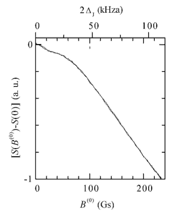
Figure 1: Experimental NOR/M_∥ (even function) in transmission of linearly polarized radiation for component ($\omega_{3}$ $P(7)$ $F^{(2)}_{2(-)}$) of ${}^{12}\mathrm{CH}_{4}$ isotope; $P\sim 3\,\mathrm{mtorr}$, $S(0)\sim 1\,\mathrm{mW}\,\mathrm{cm}^{-2}$.

Here the anomalously narrow structure clearly emerges from the background represented by wide peak having frequency analog (2). The uncommonness of the situation is that we are with pressure $P$, when collision half-width $\nu\sim 50\,\mathrm{kHza}$ [15, 16]. It is much greater $C^{\mathrm{H}}_{\mathrm{a}}$, the constant of hyperfine splitting of the line, and any structure does not emerge in NOR/Fr; at us a role of the last was played by the inverted Lamb dip, see [17, § 4.3] and [9]. HFS of NOR/Fr [13] begins to emerge with pressure on an order below ours, when $\nu\lesssim|C^{\varsigma}_{\mathrm{a}}|$. Thus we see that the collision restriction is broken in NOR/M.

Then with the purpose to level the amplitudes of both structures we went to scanning of field derivative $dS/dB^{(0)}$. By adding small sine wave modulation to slowly varied magnetic field, $B^{(0)}+\delta B^{(0)}\sin(ft)$, we extracted the first harmonics in radiation intensity, $S_{f}(B^{(0)})\simeq\delta B^{(0)}dS/dB^{(0)}$. Due to this method we have found out one more narrow structure in intensity of linearly polarized radiation. It had an inverse sign, i.e. was a dip. The next important act is transition to external cell and use of circularly polarized radiation [18, 19].

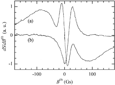
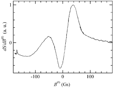
Figure 2: Derivatives of experimental NOR/M_∥ in the transmission of linearly (a) and right circularly (b) polarized radiations. At the left for component ($\omega_{3}$ $P(7)$ $F^{(2)}_{2(-)}$) of ${}^{12}\mathrm{CH}_{4}$ isotope; $\delta B^{(0)}\lesssim 10\,\mathrm{Gs}$. At the right a curve is analogous to (b), but for component ($\omega_{3}$ $P(6)$ $F^{(1)}_{2(-)}$) of ${}^{13}\mathrm{CH}_{4}$ isotope. For all curves $P\sim 2\,\mathrm{mtorr}$, $S(0)\sim 1\,\mathrm{mW}\,\mathrm{cm}^{-2}$.

Figure 2 at the left shows the typical signal derivatives for both types of radiation polarization [there are the similar experimental curves (without combining) in [18, 19]]. In the latter cited paper there was working pressure $P=3\div 6\,\mathrm{mtorr}$, when, according to [16], $\nu=55\div 100\,\mathrm{kHza}$; the recording of curves was conducted with modulation amplitude $\delta B^{(0)}=16\,\mathrm{Gs}$ and frequency $f=60\,\mathrm{Hza}$. Restoring the initial output signal $S$, we shall see, that the dips are present on both resonance curves, i.e. there are symmetrically displaced two dips [with weight $=0.25$, as it will be seen from (48)] for linearly polarized radiation and there is respectively displaced one of them (with weight $=1$) for every circularly polarized one.

We investigated only those components of fine structure of methane vibration-rotation spectrum, which hit in the limited frequency area of magnetic detuning of He-Ne laser with respect to basic component ($\omega_{3}$ $P(7)$ $F^{(2)}_{2(-)}$) of ${}^{12}\mathrm{CH}_{4}$ isotope: $|\varOmega|<3.5\,\mathrm{GHza}$. The Doppler broadening of these components will further show in (8). The next component ($\omega_{3}$ $P(6)$ $F^{(1)}_{2(-)}$) belongs to ${}^{13}\mathrm{CH}_{4}$ isotope and is detuned on $-0.9\,\mathrm{GHza}$ from basic one. One more component ($\omega_{3}$ $P(7)$ $E_{(\pm)}$) of ${}^{12}\mathrm{CH}_{4}$ isotope is detuned on $-3.0\,\mathrm{GHza}$ from basic one and has zero total spins of the subsystems with nuclei of the same type. Any sub-collision structure of its NOR/M were not experimentally revealed. At the same time, previous two mentioned components belong to different methane isotopes and, in accessible pressure range, their field spectra are quite (even qualitatively) distinctive for circularly polarized radiation and weakly (again qualitatively) distinctive for linearly polarized one. It is evidence from the typical experimental derivatives of NOR/M shown in the Figure 2 (at the right the curve for linearly polarized radiation is omitted).

It is necessary to note, that, except the methane transmission, the sub-collision structure of NOR/M was recorded in its circular birefringence [20], see below an expression (84).

First published and unsuccessful attempts [19] to interpret these structures were based on a model which is taking into account the collision in-summands in kinetic equations (4) for both resonance levels. It was considered, that the model of relaxational constants, which are taking into account only the collision out-summands in the kinetic equations (without in-summands), is insufficient for the interpretation. The authors of cited paper tried to explain the narrow structures of NOR/M for linearly polarized radiation by means of collision changing a velocity of molecules and forming the collision interference resonance [9]. One more collision model was chosen in [21], where the possibility of complete intermixing for population of hyperfine sublevels by means of deorientation collisions without velocity modification was taken into account. However, it was gradually found out (see section 5), that the collision model (as in itself and with the account of HFS) is not capable to describe adequately an observable resonance structure particularly for circularly polarized radiation.

3 Exact calculation of HFS of NOR/M_∥ in ${}^{12}\mathrm{CH}_{4}$

Let us consider the resonancely absorptive molecular gas with an operator density matrix

$$\hat{\rho}(v_{k},r_{k},t)=\left(\begin{array}[]{cc}\hat{\rho}_{m}(v_{k},r_{k},t)&\hat{\rho}_{mn}(v_{k},r_{k},t)\\ \hat{\rho}^{\dagger}_{mn}(v_{k},r_{k},t)&\hat{\rho}_{n}(v_{k},r_{k},t)\end{array}\right).$$ (3)

It depends on molecular velocity projection $v_{k}=\bm{v}\cdot\bm{k}/k$ and, similarly, coordinate one $r_{k}$ for some time $t$. The wave vector $\bm{k}$ sets the propagation direction of absorbed light. The evolution of $\hat{\rho}(v_{k},r_{k},t)$ is represented by the quantum kinetic equation with classical description of translational motion of molecules [9]:

$$(\partial_{t}+v_{k}\partial_{r_{k}})\hat{\rho}(v_{k},r_{k},t)=\hat{R}(v_{k},r_{k},t)+\hat{S}(v_{k},r_{k},t)-\mathrm{i}\left[\hat{H}(r_{k},t),\hat{\rho}(v_{k},r_{k},t)\right].$$ (4)

The statistical and dynamic summands enter in the right side of this equation. Statistical ones are represented by spontaneous one $\hat{R}(v_{k},r_{k},t)$ and collision one $\hat{S}(v_{k},r_{k},t)$. Dynamic ones are represented by a commutator with Hamiltonian $\hat{H}(r_{k},t)$. Here we are going to consider NOR/M for vibration-rotation transitions of molecules. These transitions usually hit in IR area of frequency spectrum, where it is possible to do not take $\hat{R}(v_{k},r_{k},t)$ into account completely. Let us remark only, that the spontaneous structure of NOR/M begins to be revealed in visible frequency area, when the electronic transitions are considered, and its analysis will be submitted in paper [22].

The summand $\hat{S}(v_{k},r_{k},t)$ includes components of collision excitation and relaxation for the subsystem ${[}^{m}_{n}$, extracted by absorbed radiation.

$$\hat{S}_{ij}(v_{k},r_{k},t)=\delta_{i,j}\nu_{j}\left[\tilde{N}_{j}W(v_{k})\hat{1}_{j}-\hat{\rho}_{j}(v_{k},r_{k},t)\right]-(1-\delta_{i,j})\nu\hat{\rho}_{ij}(v_{k},r_{k},t)$$ (5)

with $i$ and $j\in(m,n)$. In the presence of laser radiation tuned to ${[}^{m}_{n}$ the sufficient condition for particle number conservation is

$$\sum_{j=m,n}\langle\langle\hat{S}_{j}(v_{k},r_{k},t)\rangle\rangle_{v_{k}}=0,$$

and in its absence the mentioned condition is $\langle\langle\hat{S}_{j}(v_{k},r_{k},t)\rangle\rangle_{v_{k}}=0$. Angular brackets $\langle\ldots\rangle$ and $\langle\ldots\rangle_{x}$ (or more detailed $\langle\ldots\rangle^{(b)}_{x(a)}$) respectively mark trace and integration on $x$ (from $a$ up to $b$). For our purposes it is enough to suppose that the collisions are isotropic and excite only diagonal elements of $\hat{\rho}_{j}(v_{k},r_{k},t)$, i.e. sublevel populations of extracted $j$-levels. $\hat{1}_{j}$ — diagonal identity matrix with diagonal size $[j]=\langle\hat{1}_{j}\rangle$. The molecular excitation is characterized by Maxwell’s distribution vs. velocity (or, with reference to our field orientation, vs. its $k$-projection),

$$W(v_{k})=\mathop{\mathrm{e}}\nolimits^{-(v_{k}/v_{\mathrm{M}})^{2}}/\sqrt{\pi}v_{\mathrm{M}}$$ (6)

with integral normalization $\langle W(v_{k})\rangle_{v_{k}}=1$. Here most probable thermal velocity $v_{\mathrm{M}}=\sqrt{2k_{\mathrm{B}}T/m}$, where $m$ — molecular mass. For methane, when $T$ is room temperature, the velocity $\left.v_{\mathrm{M}}\right|_{20\,{}^{o}\mathrm{C}}\simeq 552\,\mathrm{m}\,\mathrm{s}^{-1}$. Components $\hat{\rho}_{j}(v_{k},r_{k},t)$ and $\hat{\rho}_{mn}(v_{k},r_{k},t)$ relax with frequency velocities $\nu_{j}\equiv\nu_{jj}$ and $\nu\equiv\nu_{mn}$, respectively.

$$\tilde{N}_{j}=N_{j}/[j]$$ (7)

— volumetric density of population for each sublevel of $j$-level. It makes a part from $N_{j}$ — volumetric density of total population of $j$-level (term) with sublevel number $[j]$. If to speak about methane [16] with pressure $P\sim 2\,\mathrm{mtorr}$, all its relaxational constants $\nu_{j}=\nu\sim 40\,\mathrm{kHza}\ll\omega_{\mathrm{D}}$, where Doppler half-width (at level $\mathop{\mathrm{e}}\nolimits^{-1}$ from maximum)

$$\omega_{\mathrm{D}}=kv_{\mathrm{M}}\simeq 0.16\,\mathrm{GHza}$$ (8)

for light wave length $\lambda=3.39\,\mu\mathrm{m}$. In these conditions the spectra inhomogeneously broaden and the observation of NOR is possible.

The last (dynamic) summand in the right side of the equation (4) is a commutator with Hamiltonian

$$\hat{H}(r_{k},t)=\hat{H}^{(0)}+\hat{H}^{(1)}+\hat{V}(r_{k},t)=\left(\begin{array}[]{cc}\omega_{m}+\hat{H}^{(1)}_{m}&\hat{V}_{mn}(r_{k},t)\\ \hat{V}^{\dagger}_{mn}(r_{k},t)&\omega_{n}+\hat{H}^{(1)}_{n}\end{array}\right).$$ (9)

As well as in (3), it is convenient for all operators to keep the matrix representation with operator elements, where $\hat{H}^{(0)}$ is diagonal. $\hat{H}^{(0)}$ describes a two-component subsystem ${[}^{m}_{n}$, i.e. $\hat{H}^{(0)}|j\rangle=\omega_{j}|j\rangle$. The frequency splitting of these components is optical and designated with $\omega_{mn}\equiv\omega_{m}-\omega_{n}$. Each component has HFS and $\hat{H}^{(1)}$ describes it and its nonlinear splitting in a magnetic field. $\hat{V}(r_{k},t)$ describes resonance electro-dipole interaction of these multiplet components with light, which is generated as a plane monochromatic travelling wave. In the given section we intend to describe the effect of $\hat{H}^{(1)}$ on tensor components of nonlinear-optical susceptibilities $\bm{\chi}^{(3)}$, i.e. on NOR/Fi at the end.

To exclude from consideration too large interaction of nuclear quadrupole with molecule rotation, we shall be limited to a case of molecules consisted of the half-spin nuclei. Some of these nuclei can be identical among themselves and then the molecules will have various spins modifications (i.e.  isomers), as in a subsequently considered example of molecular symmetry $\mathrm{T}_{\underline{\mathrm{d}}}$. The respective irreducible spin representations $\Gamma_{I}$ of group $\mathrm{S}_{4}\cong\mathrm{T}_{\underline{\mathrm{d}}}$ are connected one-to-one with rotation-inversion ones $\Gamma_{J_{n}}$ of group $\mathrm{T}_{\underline{\mathrm{d}}}$ for components of a fine structure of vibration-rotation spectrum in the correspondence with Pauli exclusion principle, i.e.  $\Gamma_{J_{n}}\otimes\Gamma_{I}\supseteq A_{2}$. For triply degenerated (i.e. $F_{2}$-type) $\omega_{3}$-vibration at its first exited level the Coriolis interaction substantially gives splittings ($\sim 10\,\mathrm{GHza}$) of components ($m$ is one of them). At its non-excited level the centrifugal perturbation remains only and gives splittings of components ($n$ is one of them) on an order less [23]. For either of the two optically connected vibration-rotation components ($m$ and $n$) without parity doubling, i.e. excluding $E_{(\pm)}$-components, it is possible to represent the effective Hamiltonian, combining hyperfine and Zeeman interactions, as

$$\hat{H}^{(1)}_{j}=-\sum_{\varsigma}\left(C^{\varsigma}_{\mathrm{a}}\hat{\bm{J}}_{j}+\bm{\varDelta}^{\varsigma}_{I}\right)\cdot\hat{\bm{I}}{}^{\varsigma}-\bm{\varDelta}_{J}\cdot\hat{\bm{J}}_{j}.$$ (10)

We use frequency Zeeman vectors: nuclear-spin ones $\bm{\varDelta}^{\varsigma}_{I}=\gamma^{\varsigma}_{I}\bm{B}^{(0)}$ and rotational one $\bm{\varDelta}_{J}=\gamma_{J}\bm{B}^{(0)}$. Here various gyromagnetic ratios are designated as $\gamma^{\varsigma}_{I}=g^{\varsigma}_{I}\gamma_{\mathrm{N}}$ and $\gamma_{J}=g_{J}\gamma_{\mathrm{N}}$. They are products of respective $g$-factors on a standard nuclear gyromagnetic ratio $\gamma_{\mathrm{N}}=\mu_{\mathrm{N}}/\hbar\simeq 0.762\,\mathrm{kHza}\,\mathrm{Gs}^{-1}$. $\mu_{\mathrm{N}}$ — nuclear magneton. The values of superscript $\varsigma$ are ordered and distinguish, e.g. for methane, both ordinary spin subsystem (with $I^{{}^{12}\mathrm{C}}=0$ or $I^{{}^{13}\mathrm{C}}=1/2$) and combined ${}^{1}\mathrm{H}_{4}$-subsystem. Spin modifications of the latter are respectively characterized by total spins $\left.I^{\varsigma}\right|_{\varsigma=\mathrm{H}A_{1},\mathrm{H}F_{2},\mathrm{H}E}=2,1,0$. $\hat{\bm{J}}_{j}$ with $j\in(m,n)$ and $\hat{\bm{I}}{}^{\varsigma}$ with $\varsigma\in(\varsigma_{1},\ldots,\varsigma_{k})$ (here $k$ — the number of various nuclear subsystems) respectively designate vectorial operators of rotation angular momentum of molecule and spins of its nuclear subsystems (all are measured in units of Planck constant $\hbar$) for two optically connected $(J_{j}I^{\bm{\cdot}})$-terms, where the set $I^{\bm{\cdot}}\equiv(I^{\varsigma_{1}},\ldots,I^{\varsigma_{k}})$. These methane terms have close magnetic properties, i.e.  average hyperfine constants $C^{{}^{1}\mathrm{H}}_{\mathrm{a}}\simeq 12\,\mathrm{kHza}$ [24, 13], $C^{{}^{13}\mathrm{C}}_{\mathrm{a}}\simeq-12\,\mathrm{kHza}$ [see below (26) and (90b)], rotation $g$-factor $g_{J}\simeq 0.313$ [25] and certainly both spin ones $g^{{}^{1}\mathrm{H}}_{I}\simeq 5.5854$ and $g^{{}^{13}\mathrm{C}}_{I}\simeq 1.4042$ [26].

To have an obvious model for Hamiltonian (10), we shall now write out the appropriate set of motion equations for dynamic variables in Heisenberg “representation” [1]:

$$\begin{split}\partial_{t}\hat{\bm{J}}_{j}(t)&=\hat{\bm{J}}_{j}(t)\times\left(\sum_{\varsigma}C^{\varsigma}_{\mathrm{a}}\hat{\bm{I}}{}^{\varsigma}(t)+\bm{\varDelta}^{\varsigma}_{J}\right),\\ \partial_{t}\hat{\bm{I}}{}^{\varsigma}(t)&=\hat{\bm{I}}{}^{\varsigma}(t)\times\left(C^{\varsigma}_{\mathrm{a}}\hat{\bm{J}}_{j}(t)+\bm{\varDelta}^{\varsigma}_{I}\right),\end{split}$$ (11)

and $\varsigma\in(\varsigma_{1},\ldots,\varsigma_{k})$. Here $\hat{\bm{J}}_{j}(t)=\mathop{\mathrm{e}}\nolimits^{\mathrm{i}\hat{H}^{(1)}_{j}t}\hat{\bm{J}}_{j}\mathop{\mathrm{e}}\nolimits^{\bar{\mathrm{i}}\hat{H}^{(1)}_{j}t}$ and $\hat{\bm{I}}{}^{\varsigma}(t)$ is similar. The precession ($\bm{\varDelta}_{J}\times\hat{\bm{J}}_{j}$) is a deviation from the interaction ($\bm{\varDelta}_{J}\cdot\hat{\bm{J}}_{j}$) and, as far as

$$(\bm{\varDelta}_{J}\times\hat{\bm{J}}_{j})^{2}+(\bm{\varDelta}_{J}\cdot\hat{\bm{J}}_{j})^{2}=\bm{\varDelta}^{2}_{J}\hat{\bm{J}}^{2}_{j},$$

they are two complementary characteristics of the motion. The set of equations (11) reflects our notions about a precession of nuclear-spin and rotation subsystems in a magnetic field, their hyperfine connections and balancing, and also their ruptures with growth of the magnetic field and unbalancing mentioned subsystems.

Let us designate the vector operators of total angular momentum and total nuclear spin of molecule as

$$\hat{\bm{F}}_{j}=\hat{\bm{J}}_{j}+\hat{\bm{I}}{}\quad\text{and}\quad\hat{\bm{I}}{}=\sum_{\varsigma}\hat{\bm{I}}{}^{\varsigma}.$$ (12)

For commutator $[\hat{H}^{(1)}_{j},\bm{\varDelta}_{J}\cdot\hat{\bm{F}}_{j}]=0$, it is convenient to represent (10) as

$$\hat{H}^{(1)}_{j}=\hat{h}_{j}-\bm{\varDelta}_{J}\cdot\hat{\bm{F}}_{j},$$ (13)

where

$$\hat{h}_{j}=\sum_{\varsigma}\hat{h}^{\varsigma}_{j}=-\sum_{\varsigma}\left(C^{\varsigma}_{\mathrm{a}}\hat{\bm{J}}_{j}+\bm{\varDelta}^{\varsigma}_{IJ}\right)\cdot\hat{\bm{I}}{}^{\varsigma}$$

and $\bm{\varDelta}^{\varsigma}_{IJ}\equiv\bm{\varDelta}^{\varsigma}_{I}-\bm{\varDelta}_{J}$. As well as earlier it is convenient to extract the appropriate gyromagnetic ratios, then $\bm{\varDelta}^{\varsigma}_{IJ}=\gamma^{\varsigma}_{IJ}\bm{B}^{(0)}$. Already here it is possible to notice, that HFS of NOR/M can be observed only if some $\bm{\varDelta}^{\varsigma}_{I}$ differs from $\bm{\varDelta}_{J}$. Just in this case it is possible to speak about a rupture of hyperfine connection of the appropriate nuclear spin with molecular rotation momentum. In a weak magnetic field the precession of total angular momentum takes place around of the field direction. With increasing value of the field the precession nuclear spins and molecular rotation momentum becomes more and more independent, and they cease to form the conserved total angular momentum.

We direct Cartesian unit vector $\bm{u}_{z}$ along $\bm{B}^{(0)}$, therefore $\bm{\varDelta}^{\varsigma}_{I}=\varDelta^{\varsigma}_{I}\bm{u}_{z}$, $\bm{\varDelta}_{J}=\varDelta_{J}\bm{u}_{z}$, and $\bm{\varDelta}^{\varsigma}_{IJ}=\varDelta^{\varsigma}_{IJ}\bm{u}_{z}$. The standard spherical basis is defined by covariant unit vectors [27], i.e.

$$\bm{u}_{\dot{0}{}}=\bm{u}_{z}\quad\text{and}\quad\bm{u}_{\pm\dot{1}{}}=\mp(\bm{u}_{x}\pm i\bm{u}_{y})/\sqrt{2}.$$ (14)

Contravariant unit vectors $\bm{u}_{\underset{\scriptstyle\dot{}}{q}{}}\equiv\bm{u}^{*}_{\dot{q}{}}=(-1)^{q}\bm{u}_{\dot{\bar{q}}{}}$, so $\bm{u}_{\dot{q}^{\prime}{}}\cdot\bm{u}_{\underset{\scriptstyle\dot{}}{q}{}}=\delta_{q^{\prime},q}$. Contra- and co-variant magnitudes have under- and over-dotted indices, respectively. The complex conjugation and its generalization, the Hermitian one, are respectively designated with superscript asterisk ^∗ and dagger ^†.

Unlike [21], using $F_{j}M$-basis, we shall choose completely split basis of wave functions, i.e.

$$|j\mu^{\bm{\cdot}}M\rangle=|(J_{j}I^{\bm{\cdot}})\mu^{\bm{\cdot}}M\rangle\equiv|J_{j}M-\mu\rangle\prod_{\varsigma}|I^{\varsigma}\mu^{\varsigma}\rangle,$$ (15a)

where $$M\equiv\langle j\mu^{\bm{\cdot}}M|\hat{F}_{jz}|j\mu^{\bm{\cdot}}M\rangle$$ and the set of nuclear spin projections

$$\mu^{\bm{\cdot}}\equiv(\mu^{\varsigma_{1}},\ldots,\mu^{\varsigma_{k}}),\quad\mu=\sum_{\varsigma}\mu^{\varsigma},\quad|\mu^{\varsigma}|\leq I^{\varsigma};$$ (15b)

In this basis the Hamilton operator $\hat{H}^{(1)}_{j}$ has the following matrix representation

$$\underline{\hat{H}}{}^{(1)}_{jM}=\sum_{\varsigma}\underline{\hat{h}}{}^{\varsigma}_{jM}-\varDelta_{J}M,$$

where

$$\left(\underline{\hat{h}}{}^{\varsigma}_{jM}\right)_{\mu^{\bm{\cdot}\prime}\mu^{\bm{\cdot}}}\equiv\langle j\mu^{\bm{\cdot}\prime}M|\hat{h}{}^{\varsigma}_{j}|j\mu^{\bm{\cdot}}M\rangle$$

with

$$\underline{\hat{h}}{}^{\varsigma}_{jM}=-\left(C^{\varsigma}_{\mathrm{a}}\bm{J}^{\dagger}_{j,M-\underline{\hat{I}}{}_{z}}+\bm{\varDelta}^{\varsigma}_{IJ}\right)\cdot\underline{\hat{\bm{I}}}{}^{\varsigma}.$$ (16)

Matrix elements of covariant rotation operator components, $\hat{J}_{j\dot{q}{}}=\hat{\bm{J}}_{j}\cdot\bm{u}_{j\dot{q}{}}$, are

$$J_{j\dot{q}{}M} \equiv\langle J_{j}M^{\prime}|\hat{J}_{j\dot{q}{}}|J_{j}M\rangle=\sqrt{\hat{\bm{J}}_{j}^{2}}\langle J_{j}M^{\prime}|J_{j}M\,1q\rangle$$

$$=\delta_{M^{\prime},M+q}\left(\delta_{q,0}M-q\delta_{|q|,1}\sqrt{(\hat{\bm{J}}_{j}^{2}-M^{\prime}M)/2}\right).$$ (17)

Here $\hat{\bm{J}}{}^{2}_{j}\equiv J_{j}(J_{j}+1)$ and it is similar for spin operators $\hat{\bm{I}}{}^{\varsigma}$.

E.g., when $I=1$ (and $J\geq I$), the matrix (16) is usually obtained with sizes $3\times 3$. Its eigenvalues are numbered at us by an index $\tilde{\mu}=1,0,\bar{1}$. For convenience we shall cite explicit expressions for three real roots of reduced (i.e. without a quadratic summand) cubic equation

$$y^{3}+py+q=0$$

in “irreducible” case, i.e., when a discriminant $D=(p/3)^{3}+(q/2)^{2}<0$ and therefore $p<0$. The trigonometrical expression for the roots, ordered in the way appropriated for us, is

$$y_{\tilde{\mu}}=2R\cos\left(\frac{\alpha-2\pi\tilde{\mu}}{3}\right),$$

where $R=\sqrt{\bar{p}/3}$ and $\cos\alpha=\bar{q}/2R^{3}$ with $0\leq\alpha\leq\pi$.

When $I\geq 2$ the exact eigenvalues for (16) are determined with a solution of the appropriate algebraic equation (of degree $[I]$, if $J\geq I$), e.g., with the help of theta-functions (with the displaced arguments) $\theta[{}^{\bm{a}}_{\bm{b}}](\bm{z},\hat{\bm{\varOmega}})$, see [32].

We shall designate the found eigenvalues as $z_{j_{l}}$, where a set of quantum numbers $j_{l}\equiv j\tilde{\mu}^{\bm{\cdot}}_{l}M_{l}$. In our case, for a determination of wave eigenfunctions appropriated to them, one can use projective operators,

$$\hat{P}^{(1)}_{j_{l}}=\prod\limits_{j_{k}\neq j_{l}}\frac{z_{j_{k}}\hat{1}_{j}-\hat{H}^{(1)}_{j}}{z_{j_{k}}-z_{j_{l}}},$$ (18)

constructed on the basis of minimum equation, see [33, appl. 5] and [29, Chap. IV]. Another (equivalent) way of their explicit construction is based on use for the operator (10) a resolvent [34, § 5.8]:

$$\hat{R}^{(1)}_{j}(z)=(z\hat{1}_{j}-\hat{H}^{(1)}_{j})^{-1}=\sum_{j_{l}}\frac{\hat{P}^{(1)}_{j_{l}}}{z-z_{j_{l}}}.$$ (19)

It is visible, that the projectors $\hat{P}^{(1)}_{j_{l}}$ are its residues, i.e.

$$\hat{P}^{(1)}_{j_{l}}=\mathop{\mathrm{Res}}\limits_{j_{l}}\,\hat{R}^{(1)}_{j}(z)=\oint\limits_{{\scriptscriptstyle j_{l}}\raisebox{-1.04996pt}{${\displaystyle\circlearrowleft}$}}\frac{dz}{2\pi\mathrm{i}}\hat{R}^{(1)}_{j}(z).$$ (20)

Here spectral parameter $z\in\mathbb{C}$, and integration path $\circlearrowleft$ enclose only one point $z_{j_{l}}$ of spectrum for operator $\hat{H}^{(1)}_{j}$.

As a result we come to a basis set of wave functions, simultaneously diagonalizing the Hamiltonians of hyperfine and Zeeman interactions, i.e.

$$|j\tilde{\mu}^{\bm{\cdot}}M\rangle=\sum_{\mu^{\bm{\cdot}}}|j\mu^{\bm{\cdot}}M\rangle(\hat{\mathcal{U}}_{jM})_{\mu^{\bm{\cdot}}\tilde{\mu}^{\bm{\cdot}}},$$ (21a)

where the set of nuclear spin quasi-projections

$$\tilde{\mu}^{\bm{\cdot}}\equiv(\tilde{\mu}^{\varsigma_{1}},\ldots,\tilde{\mu}^{\varsigma_{k}}),\quad|\tilde{\mu}^{\varsigma}|\leqslant I^{\varsigma}.$$ (21b)

It is convenient to choose them from the same set as (15b). As an example let us consider the methane isotope ${}^{12}\mathrm{CH}_{4}$, where there is only one spin subsystem (of hydrogen nuclei). We shall be limited to a case, when its total spin $I=I^{\mathrm{H}}=1$, therefore $\tilde{\mu}=\tilde{\mu}^{\mathrm{H}}$ and $\mu=\mu^{\mathrm{H}}$. Adding spin-spin interaction to the spin-rotation one, it is possible to represent more precisely the reduced form of total Hamiltonian [24, 35, 36] as

$$\hat{H}^{(1)}_{j}=\hat{h}_{jM}-\bm{\varDelta}_{J}\cdot\hat{\bm{F}}_{j}=-C^{\mathrm{H}}_{1j}\hat{\bm{J}}_{j}\cdot\hat{\bm{I}}{}\\ -C^{\mathrm{H}}_{2j}(\hat{\bm{J}}_{j}\cdot\hat{\bm{I}})^{2}-\gamma_{\mathrm{N}}(g_{J}\hat{\bm{J}}_{j}+g^{\mathrm{H}}_{I}\hat{\bm{I}})\cdot\bm{B}^{(0)}.$$ (22)

While the magnetic dependence of its spectrum

$$H^{(1)}_{j\tilde{\mu}M}=h_{j\tilde{\mu}M}-\varDelta_{J}M$$ (23)

is nearly linear from $B^{(0)}=0$ and $(g_{J}\hat{\bm{J}}_{j}+g^{\mathrm{H}}_{I}\hat{\bm{I}})\simeq g_{F}\hat{\bm{F}}_{j}$, it is possible to use $g$-factors

$$g_{F}=\frac{g^{\mathrm{H}}_{I}+g_{J}}{2}+g^{\mathrm{H}}_{IJ}\frac{I(I+1)-J(J+1)}{2F(F+1)},$$ (24)

where $g^{\mathrm{H}}_{IJ}\equiv g^{\mathrm{H}}_{I}-g_{J}$, and similarly for gyromagnetic ratios $\gamma_{F}=g_{F}\gamma_{\mathrm{N}}$. From here, e.g., for simultaneously integer (or half-integer) $J$ and $I$, $g$-factor difference

$$g_{F=J}-g_{J}=\frac{g^{\mathrm{H}}_{IJ}I(I+1)}{2J(J+1)}\geq 0.$$ (25)

Taking hyperfine intervals (i.e. experimentally measured splittings in the upper and lower hyperfine multiplets with $B^{(0)}=0$) from [13], we shall get the hyperfine constants

$$\begin{split}C^{\mathrm{H}}_{1m}&=11.66\,\mathrm{kHza},\quad C^{\mathrm{H}}_{2m}=0.22\,\mathrm{kHza},\\ C^{\mathrm{H}}_{1n}&=11.58\,\mathrm{kHza},\quad C^{\mathrm{H}}_{2n}=0.17\,\mathrm{kHza}.\end{split}$$ (26)

Now let us see in Figure 3, showing magnetic dependence of all $M$-sublevels in diagonalizing basis. As we shall see further, the features of $H^{(1)}_{j\tilde{\mu}M}$, shown on it above, and $h_{j\tilde{\mu}M}$, shown on it below, correspond to the features of spectrum of NOR/M_∥ in cases of linearly and circularly polarized radiations respectively.

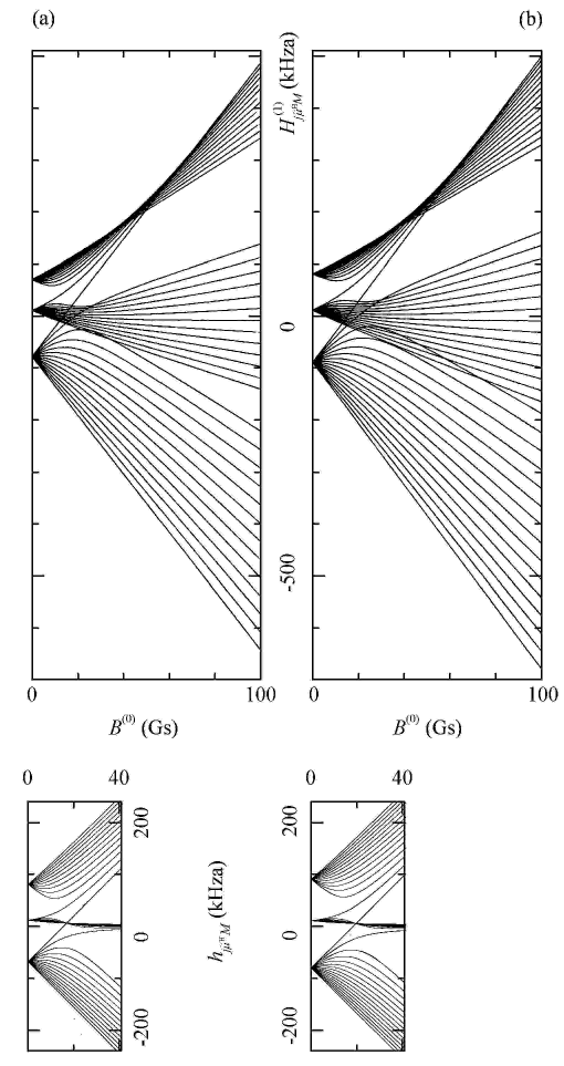
Figure 3: Exact calculated magnetic splittings (23) for both hyperfine multiplets ($J_{j}I^{\mathrm{H}}$) of component ($\omega_{3}$ $P(7)$ $F^{(2)}_{2(-)}$) of ${}^{12}{\mathrm{CH}}_{4}$ isotope: (a) for upper one with $J_{\mathrm{m}}=6$ and $I^{\mathrm{H}}=1$, (b) for lower one with $J_{\mathrm{n}}=7$ and $I^{\mathrm{H}}=1$.

The graphs of sublevels only for positive fields are shown. It is possible to restore a dependence of sublevels on negative fields if we take into account that $H^{(1)}_{j\tilde{\mu}M}(-B^{(0)})=H^{(1)}_{j\tilde{\mu}\bar{M}}(B^{(0)})$, i.e.  the whole splitting picture comes from a mirror reflection with respect to ordinate axis. It is visible that the one weakly differs at upper (a) and lower (b) hyperfine multiplets. With large $B^{(0)}$ (after all crossings) the sets of sublevels $(M)_{\tilde{\mu}}$ are ordered from top to bottom, as [$(-J_{j}-1,-J_{j},\ldots,J_{j}-1)_{\bar{1}}$; $(-J_{j},-J_{j}+1,\ldots,J_{j})_{0}$; $(-J_{j}+1,-J_{j}+2,\ldots,J_{j}+1)_{1}$] on graphs shown above, and as [$(J_{j}-1,J_{j}-2,\ldots,-J_{j}-1)_{\bar{1}}$; $(J_{j},J_{j}-1,\ldots,-J_{j})_{0}$, $(-J_{j}+1,-J_{j}+2,\ldots,J_{j}+1)_{1}$] on graphs shown below. In these sets there are repulsing (anti-crossing) of sublevels with equal $M$ and unequal $\tilde{\mu}$. For anyone $J_{j}$ all magnetic sublevels with unequal $M$ and equal $\tilde{\mu}$ are crossed with $B^{(0)}=0$, and separately for each $\tilde{\mu}$. When the field $B^{(0)}$ is close to zero, we have an approximation, $(F_{j}-J_{j})\simeq\tilde{\mu}_{j}$, where $\hat{\bm{F}}{}_{j}$ is defined in (12). With increasing the field all sublevels, shown in Figure 3 above, diverge and we have another approximation, $\mu_{j}\simeq\tilde{\mu}_{j}$.

In both upper graphs of Figure 3 the greatest number of crossings in nonzero fields is observed in single twist area for the fan of magnetic sublevels of (upper) component with $\tilde{\mu}=-1$, exactly with

$${}^{\mathrm{H}}B^{(0)}_{\mathrm{cr}}\simeq\pm C^{\mathrm{H}}_{\mathrm{a}}/\gamma_{J},$$ (27)

when $J\lesssim g^{\mathrm{H}}_{IJ}/g_{J}$ with $g^{\mathrm{H}}_{IJ}\geq 0$. With greater $J$, when the factor $g_{F=J-1}$ in (24) changes a sign, the twist area disappears.

In both lower graphs of Figure 3 our attention is attracted by the feature located at nonzero fields in a point of twist for fan of magnetic sublevels of (middle) component with $\tilde{\mu}=0$:

$${}^{\mathrm{H}}B^{(0)}_{\mathrm{Ncr}}\simeq\pm C^{\mathrm{H}}_{\mathrm{a}}J/\gamma^{\mathrm{H}}_{IJ}$$ (28)

Non-repulsed magnetic sublevel of (lower) component with $\tilde{\mu}=1$ also passes through it.

In the basis chosen by us for diagonalizing wave functions with anyone $B^{(0)}$ all states would be stationary at absence of collision pumping and relaxation. At us, at their presence, they will be equilibrium, i.e. balanced on these processes. All possible transitions between these states will be purely optical, due to resonance electro-dipole interaction with a light field $\bm{E}(r_{k},t)$, exactly

$$\hat{V}_{mn}(r_{k},t) =-\hat{\bm{d}}{}^{mn}\cdot\bm{E}(r_{k},t)/\hbar$$

$$=-\sum_{q}\hat{d}^{mn}_{\dot{q}{}}E_{\underset{\scriptstyle\dot{}}{q}{}}(r_{k},t)/\hbar.$$ (29)

According to Wigner-Eckert factorizational theorem (see [27] or expression (62) in [6]), vector operator of electro-dipole moment of a transition can be connected with covariant components of standard operator, affecting only rotation variable, namely,

$$\hat{\bm{d}}{}^{mn}=\tilde{d}_{mn}\hat{\bm{T}}{}^{mn}=\tilde{d}_{mn}\sum_{q}\hat{T}^{mn}_{\dot{q}{}}\bm{u}_{\underset{\scriptstyle\dot{}}{q}{}},$$ (30)

and trace normalization is

$$\langle\hat{T}^{mn\dagger}_{\dot{q}{}^{\prime}}\hat{T}^{mn}_{\dot{q}{}}\rangle\equiv\mathop{\mathrm{tr}}\left(\hat{T}^{mn\dagger}_{\dot{q}{}^{\prime}}\hat{T}^{mn}_{\dot{q}{}}\right)=\delta_{q^{\prime},q}.$$ (31)

The physical characteristics of operator $\hat{\bm{d}}$ is determined with its modified $\tilde{d}_{mn}$. The matrix elements of covariant spherical components of standard rotation operator in $JM_{J}$-basis are

$$T^{mn}_{\varkappa\dot{q}M}\equiv{}_{\mathrm{s}}T^{J_{m}J_{n}}_{\varkappa\dot{q}M} =\langle J_{m}M^{\prime}|\hat{T}^{mn}_{\varkappa\dot{q}{}}|J_{n}M\rangle$$

$$\equiv\frac{[J_{m}\|\hat{\bm{T}}^{(J)mn}_{\varkappa}\|J_{n}]}{\sqrt{[J_{m}]}}\langle J_{m}M^{\prime}|\varkappa q~{}J_{n}M\rangle$$ (32)

$$=\sqrt{\frac{[\varkappa]}{[J_{m}]}}\langle J_{m}M^{\prime}|J_{n}M~{}\varkappa q\rangle.$$ (33)

At us $[J_{j}]\equiv 2J_{j}+1$. Here we have defined another reduced matrix element $[J_{m}\|\hat{\bm{T}}^{(J)mn}_{\varkappa}\|J_{n}]$. In this particular case we have

$$[J_{m}\|\hat{\bm{T}}^{(J)mn}_{\varkappa}\|J_{n}]=(-1)^{-J_{m}+\varkappa+J_{n}}\sqrt{[\varkappa]}.$$ (34)

It is convenient also to use extra operators (to standard one)

$$\begin{split}{}_{\mathrm{e}}\hat{\bm{T}}{}^{J_{m}J_{n}}_{\varkappa}&=(-1)^{-J_{m}+\varkappa+J_{n}}{}_{\mathrm{s}}\hat{\bm{T}}{}^{J_{m}J_{n}}_{\varkappa},\\ {}_{\mathrm{e}}T^{J_{m}J_{n}}_{\varkappa\dot{q}M}&=\sqrt{\frac{[\varkappa]}{[J_{m}]}}\langle J_{m}M^{\prime}|\varkappa q~{}J_{n}M\rangle,\end{split}$$ (35)

coordinated with the definition (32) on phase. Owing to that, we now have

$$[J_{m}\|{}_{\mathrm{e}}\hat{\bm{T}}^{(J)mn}_{\varkappa}\|J_{n}]=\sqrt{[\varkappa]}.$$ (36)

The subscript “s” is sometimes omitted, as in (32) and (34). Also sometimes the subscript “$\varkappa$”, if it is equal $1$, is generally omitted, as in (30) and (31). Owing to the orthogonality of Wigner coefficients a permutation is possible, namely, $\langle J_{m}M^{\prime}|J_{n}M~{}\varkappa q\rangle=\langle J_{n}M~{}\varkappa q|J_{m}M^{\prime}\rangle$. With large $J_{j}$ an approximation by means of $d$-functions [27] is possible:

$$\langle J_{m}M^{\prime}|J_{n}M~{}\varkappa q\rangle\simeq d^{\varkappa}_{q,J_{mn}}(\theta_{JM})\delta_{M^{\prime},M+q}\varepsilon^{(\varDelta)}_{J_{m},J_{n},\varkappa}.$$ (37)

Here $\cos\theta_{JM}=M/\sqrt{\hat{\bm{J}}{}^{2}_{n}}$. $J_{mn}\equiv J_{m}-J_{n}=-1,0,1$ (or P,Q,R). If triangle condition for ($J_{m},J_{n},\varkappa$) is true, then function $\varepsilon^{(\varDelta)}_{J_{m},J_{n},\varkappa}$ is equal $1$, else $0$ [27, Chap. 5 § 8]. The matrix elements of covariant operator components of electro-dipole moment are now written as

$$d^{mn}_{\dot{q}{}M}=\tilde{d}_{mn}T^{mn}_{\dot{q}{}M}\simeq d_{mn}d^{1}_{q,J_{mn}}(\theta).$$ (38)

We have

$$\tilde{d}_{nm}=(-1)^{J_{mn}}\tilde{d}^{*}_{mn}$$

and, for $d_{mn}=\sqrt{3/[J_{m}]}\tilde{d}_{mn}$,

$$d_{nm}=(-1)^{J_{mn}}d^{*}_{mn}\sqrt{[J_{m}]/[J_{n}]}.$$

Take note, that for contravariant components we have

$$\hat{d}^{nm}_{\underset{\scriptstyle\dot{}}{q}{}}\equiv\hat{d}^{mn\dagger}_{\dot{q}{}}=(-1)^{q}\hat{d}^{nm}_{\dot{\bar{q}}{}},$$

but

$$\hat{T}^{nm}_{\underset{\scriptstyle\dot{}}{q}{}}=(-1)^{J_{mn}}\hat{T}^{mn\dagger}_{\dot{q}{}}=(-1)^{q}\hat{T}^{nm}_{\dot{\bar{q}}{}}.$$

Before to consider selection rules for ours electro-dipole transition in an arbitrary magnetic field, we shall write out the reduced matrix element of standard rotation operator for $FM$-basis:

$$[(J^{\prime}I)F^{\prime}\|T^{(J)mn}_{\varkappa}\|(JI)F]=(-1)^{J^{\prime}+I+F^{\prime}}\Pi_{F^{\prime}\varkappa F}\left\{\begin{array}[]{ccc}F^{\prime}&\varkappa&F\\ J&I&J^{\prime}\end{array}\right\}$$ (39)

Here $\Pi_{xy\ldots}\equiv\sqrt{[xy\ldots]}$ with $[xy\ldots]\equiv[x][y]\ldots$. The case $I=\varkappa=1$ is interesting to us, when exact expression for

$$\left([(J^{\prime}1)F^{\prime}\|T^{(J)mn}_{1}\|(J1)F]_{\tilde{\mu}^{\prime},\tilde{\mu}}\right)=\sqrt{3}\left(\begin{array}[]{ccc}\sqrt{\frac{2J+3}{2J+1}}&-\frac{1}{J}&\frac{1}{J\sqrt{4J^{2}-1}}\\ 0&\frac{\sqrt{J^{2}-1}}{J}&-\frac{1}{J}\\ 0&0&\sqrt{\frac{2J-3}{2J-1}}\end{array}\right).$$ (40)

Here both matrix subscripts, $\tilde{\mu}^{\prime}=F^{\prime}-J^{\prime}$ and $\tilde{\mu}=F-J$, accept values $1,0,-1$ beginning at left upper angle of the matrix.

Now we shall define in (29) an electrical field of resonance absorbed IR radiation by means of slowly varying contravariant circular components $E^{(\omega)}_{\underset{\scriptstyle\dot{}}{q}{}}(r_{k})$ of plane monochromatic travelling wave [cp. with (1)]

$$\begin{split}\bm{E}(r_{k},t)&=\mathop{\mathrm{Re}}\left(\bm{E}^{(\omega)}(r_{k})\mathop{\mathrm{e}}\nolimits^{\mathrm{i}(kr_{k}-\omega t)}\right)\\ \text{and}\quad\bm{E}^{(\omega)}(r_{k})&=\sum_{q}E^{(\omega)}_{\underset{\scriptstyle\dot{}}{q}{}}(r_{k})\bm{u}_{\dot{q}{}}.\end{split}$$ (41)

Here $E^{(\omega)}_{\underset{\scriptstyle\dot{}}{q}{}}(r_{k})=E^{(\omega)}_{\underset{\scriptstyle\dot{}}{q}{}}(0)\mathop{\mathrm{e}}\nolimits^{\mathrm{i}2\pi\chi_{q}kr_{k}}$ with wave number $k_{q}=n_{q}k\simeq(1+2\pi\chi_{q})k$, $k=2\pi/\lambda$. Effective susceptibility $\chi_{q}$ and refraction factor $n_{q}$ have imaginary components due to a small absorption of gas medium. The factor (or inverse length) of this absorption is

$$\alpha_{q}=1/L_{\mathrm{a}}=2kn^{\prime\prime}_{q}\simeq 4\pi k\chi^{\prime\prime}_{q}.$$ (42)

Normalized (on pressure) factor of linear absorption of methane [37] for $\lambda=3.39\,\mu\mathrm{m}$ is

$$\alpha^{(1)P}=\alpha^{(1)}/P\simeq 0.18\,\mathrm{cm}^{-1}\,\mathrm{torr}^{-1}.$$ (43)

Hence, when pressure $P\sim 1\,\mathrm{mtorr}$, the absorption length $L_{\mathrm{a}}\sim 56\,\mathrm{m}$ and $kL_{\mathrm{a}}\gg 1$. The absolute value of light detuning $|\varOmega|\ll\omega_{mn}$ and it is possible to use resonance approximation.

With parallel orientation of fields $\bm{e}\perp\bm{k}\parallel\bm{B}^{(0)}$, where $\bm{e}$ is defined in (2b). We suppose, that the radiation polarized on right circle, has $q=1$, i.e. positive spirality. For a radiation polarized linearly, it is convenient to define a rotation angle $\theta$ of polarization plane, and a ratio $\psi$ of small semi-axis of polarization ellipse to large one:

$$\theta+\mathrm{i}\psi=\pi kr_{k}(\chi_{1}-\chi_{\bar{1}})=kr_{k}(n_{1}-n_{\bar{1}})/2.$$ (44)

The equation can be expanded with the account of nonlinear-optical corrections.

The interaction (29) brings to a small nonlinear absorption of polarized laser radiation, having intensity (i.e. surface density of radiation power)

$$S_{s}(r_{k})=|\bm{E}^{(\omega)}(r_{k})|^{2}c/8\pi.$$

A variation of the intensity after passage of absorptive gas cell is

$$\delta S_{s}(L)=S_{s}(L)-S_{s}(0)=\langle\delta S_{v}(r_{k})\rangle_{r_{k}}^{(L)}$$

$$=-\langle\langle\bm{E}(r_{k},t)\cdot\frac{\partial_{t}}{T}\bm{P}(r_{k},t)\rangle_{t}^{(T)}\rangle_{r_{k}}^{(L)}\simeq-\frac{\omega}{2}\mathop{\mathrm{Im}}\langle\bm{E}^{(\omega)*}(r_{k})\cdot\bm{P}^{(\omega)}(r_{k})\rangle^{(L)}_{r_{k}}\leq 0.$$

Here volume density of radiation power

$$\delta S_{v}(r_{k})=2\hbar\omega\mathop{\mathrm{Im}}\langle\hat{V}^{(\omega)\dagger}_{mn}(r_{k})\langle\hat{\rho}^{(\omega)}_{mn}(v_{k},r_{k})\rangle_{v_{k}}\rangle,$$

as we shall see from (51) and (52). The integral with respect to $r_{k}$ and $t$-averaging are taken from volume density of absorption power, $\bm{E}(r_{k},t)\cdot\partial_{t}\bm{P}(r_{k},t)$, spent by light field on polarization variation of gas medium. $L$ practically is a length of absorptive cell and the average is taken on time period of light, i.e. $T=2\pi/\omega$.

$$\delta S_{s}(L)\simeq\delta S_{s}^{(1)}(L)+\delta S_{s}^{(3)}(L).$$

Here the contributions of linear and cubic (on amplitude of electric field of light) components of polarization of gas medium are only retained. If relative linear absorption $\tilde{\alpha}^{(1)}_{nm}r_{k}\ll 1$ and saturation parameter $\varkappa\ll 1$, a relative variation of transmission is also small and its expansion on $\varkappa$ looks as

$$\delta S_{s}(L)/S_{s}(0)\simeq-\alpha L<0$$ (45a)

with effective absorption factor (i.e. line density of absorption)

$$\alpha=\sum_{q}\alpha_{q}|e_{\underset{\scriptstyle\dot{}}{q}{}}|^{2}\simeq\alpha^{(1)}+\alpha^{(3)}$$

$$=\sum_{q}(\alpha^{(1)}_{q}+\alpha^{(3)}_{q})|e_{\underset{\scriptstyle\dot{}}{q}{}}|^{2}\simeq-\tilde{\alpha}^{(1)}_{nm}(s^{(1)}+\varkappa s^{(3)}/2).$$ (45b)

Factor $1/2$ at $\varkappa$ is extracted by analogy with nondegenerate two-level case, when saturation expansion $(1+\varkappa)^{-1/2}\simeq 1-\varkappa/2$; see [9]. As well in our case, it is expected that the amplitudes of amplification functions $s^{(i)}$ (modulo) are close to $1$, i.e.  $s^{(i)}$ are normalized. Linear-optical resonance with magnetic scanning (LOR/M) is

$$s^{(1)}\equiv s^{(1)}_{(\bm{e})}=-\mathop{\mathrm{Re}}[\tilde{\bm{X}}{}^{(1)mn}\,:\,\bm{e}^{*}\otimes\bm{e}]$$

$$=-\mathop{\mathrm{Re}}\sum_{(q_{i})}\tilde{X}^{(1)mn}_{\underset{\scriptstyle\dot{}}{q}{}_{0}\dot{q}{}_{1}}e^{*}_{\underset{\scriptstyle\dot{}}{q}{}_{0}}e_{\underset{\scriptstyle\dot{}}{q}{}_{1}}=-\sum_{q}\tilde{X}^{(1)mn\prime}_{\underset{\scriptstyle\dot{}}{q}{}\dot{q}{}}|e_{\underset{\scriptstyle\dot{}}{q}{}}|^{2}.$$ (46)

NOR/M is (in vector designations and component by component)

$$s^{(3)}\equiv s^{(3)}_{(\bm{e})} =\tilde{\bm{X}}{}^{(3)mn}\,\underset{\displaystyle\cdot}{\vdots}\,\bm{e}^{*}\otimes\bm{e}\otimes\bm{e}^{*}\otimes\bm{e}$$

$$=\sum_{(q_{i})}\tilde{X}^{(3)mn}_{\underset{\scriptstyle\dot{}}{q}{}_{0}\dot{q}{}_{1}\underset{\scriptstyle\dot{}}{q}{}_{2}\dot{q}{}_{3}}e^{*}_{\underset{\scriptstyle\dot{}}{q}{}_{0}}e_{\underset{\scriptstyle\dot{}}{q}{}_{1}}e^{*}_{\underset{\scriptstyle\dot{}}{q}{}_{2}}e_{\underset{\scriptstyle\dot{}}{q}{}_{3}}\quad(\in\mathbb{R}).$$ (47)

NOR/M_∥ is

$$s^{(3)}_{\parallel}=\sum_{q=\pm 1}\left[\tilde{\bm{\between}}{}^{m}_{nq}|e_{\underset{\scriptstyle\dot{}}{q}{}}|^{2}+\left(\tilde{\bm{\vee}}{}^{m}_{nq}+\tilde{\bm{\wedge}}{}^{m}_{nq}\right)|e_{\underset{\scriptstyle\dot{}}{\bar{q}}{}}|^{2}\right]|e_{\underset{\scriptstyle\dot{}}{q}{}}|^{2}$$

$$\equiv\sum_{q=\pm 1}\left[\tilde{X}^{(3)mn}_{\underset{\scriptstyle\dot{}}{q}{}\dot{q}{}\underset{\scriptstyle\dot{}}{q}{}\dot{q}{}}|e_{\underset{\scriptstyle\dot{}}{q}{}}|^{2}+\left(\tilde{X}^{(3)mn}_{\underset{\scriptstyle\dot{}}{q}{}\dot{q}{}\underset{\scriptstyle\dot{}}{\bar{q}}{}\dot{\bar{q}}{}}+\tilde{X}^{(3)mn}_{\underset{\scriptstyle\dot{}}{q}{}\dot{\bar{q}}{}\underset{\scriptstyle\dot{}}{\bar{q}}{}\dot{q}{}}\right)|e_{\underset{\scriptstyle\dot{}}{\bar{q}}{}}|^{2}\right]|e_{\underset{\scriptstyle\dot{}}{q}{}}|^{2}$$

$$=\tilde{\bm{\between}}{}^{m}_{n1}|e_{\underset{\scriptstyle\dot{}}{1}{}}|^{4}+\tilde{\bm{\between}}{}^{m}_{n\bar{1}}|e_{\underset{\scriptstyle\dot{}}{\bar{1}}{}}|^{4}+2|e_{\underset{\scriptstyle\dot{}}{1}{}}e_{\underset{\scriptstyle\dot{}}{\bar{1}}{}}|^{2}\left(\tilde{\bm{\vee}}{}^{m\prime}_{n1}+\tilde{\bm{\wedge}}{}^{m\prime}_{n1}\right);$$ (48)

the convenient graphic designations are here introduced. NOR/M_⟂ is

$$s^{(3)}_{\perp}=\tilde{\bm{\between}}{}^{m}_{n0}\equiv\tilde{X}^{(3)mn}_{\underset{\scriptstyle\dot{}}{0}{}\dot{0}{}\underset{\scriptstyle\dot{}}{0}{}\dot{0}{}}.$$ (49)

The meaning of subscripts $\parallel$ and $\perp$ is above defined on p. 1. In both cases $\bm{u}_{z}=\bm{B}^{(0)}/B^{(0)}$. Here we use the components of two modified $X$-tensors,

$$\begin{split}\tilde{\bm{X}}{}^{(1)mn}&=\left.\bm{X}^{(1)mn}\right/[p]\prod_{\varsigma}[I^{\varsigma}]\\ \text{and}\quad\tilde{\bm{X}}{}^{(3)mn}&=\left.\bm{X}^{(3)mn}\,[J_{m}]\right/3[p]\prod_{\varsigma}[I^{\varsigma}].\end{split}$$ (50)

It is visible that their normalizing factors are different. Original $X$-tensors are defined slightly further in (55). Their explicit construction turns out from the short Maxwell equations in approximation of slowly varying amplitudes [38], i.e.

$$\partial_{r_{k}}\bm{E}^{(\omega)}(r_{k})=\mathrm{i}2\pi k\bm{P}^{(\omega)}(r_{k}).$$

For that it is required to calculate the volume density of light-induced (on light frequency) electro-dipole momentum (or electrical polarization) of our gas medium, namely,

$$\bm{P}(r_{k},t) =\left\langle\hat{\bm{d}}\langle\hat{\rho}(v_{k},r_{k},t)\rangle_{v_{k}}\right\rangle=2\mathop{\mathrm{Re}}\left\langle\hat{\bm{d}}{}^{mn\dagger}\langle\hat{\rho}_{mn}(v_{k},r_{k},t)\rangle_{v_{k}}\right\rangle$$

$$=\mathop{\mathrm{Re}}\left(\bm{P}^{(\omega)}(r_{k})\mathop{\mathrm{e}}\nolimits^{\mathrm{i}(kr_{k}-\omega t)}\right)$$

$$\text{and}\quad\bm{P}^{(\omega)}(r_{k}) =\sum_{q}P^{(\omega)}_{\underset{\scriptstyle\dot{}}{q}{}}(r_{k})\bm{u}_{\dot{q}{}}=2\left\langle\hat{\bm{d}}{}^{mn\dagger}\langle\hat{\rho}^{(\omega)}_{mn}(v_{k},r_{k})\rangle_{v_{k}}\right\rangle.$$ (51)

Here $\hat{\rho}(v_{k},r_{k},t)$ is the operator density matrix of gas medium and its light-induced non-diagonal component $\hat{\rho}_{mn}(v_{k},r_{k},t)\simeq\hat{\rho}^{(\omega)}_{mn}(v_{k},r_{k})\mathop{\mathrm{e}}\nolimits^{\mathrm{i}(kr_{k}-\omega t)}$. Passing in the equation (4) to the representation of interaction on

$$\hat{V}^{\prime}(r_{k},t)=\mathop{\mathrm{e}}\nolimits^{\mathrm{i}(\hat{H}^{(0)}+\hat{H}^{(1)})t}\hat{V}(r_{k},t)\mathop{\mathrm{e}}\nolimits^{\bar{\mathrm{i}}(\hat{H}^{(0)}+\hat{H}^{(1)})t}$$

(see [1, Chap. VIII § 14 and Chap. XVII § 1]), using shortened form of the equation, when $v_{k}\partial_{r_{k}}\sim v_{\mathrm{M}}/L_{\mathrm{a}}\ll\nu$, and being then limited its slow component in resonance condition ($|\varOmega|\ll\omega_{mn}$), when

$$\hat{V}^{\prime}_{mn}(r_{k},t)\simeq\hat{V}^{(\varOmega)}_{mn}(r_{k},t)\mathop{\mathrm{e}}\nolimits^{\mathrm{i}(kr_{k}-\varOmega t)},$$

but $\hat{V}^{\prime}_{jj}(r_{k},t)=0$, and

$$\hat{V}^{(\varOmega)}(r_{k},t)\equiv\mathop{\mathrm{e}}\nolimits^{\mathrm{i}\hat{H}^{(1)}t}\hat{V}^{(\omega)}(r_{k})\mathop{\mathrm{e}}\nolimits^{\bar{\mathrm{i}}\hat{H}^{(1)}t}$$

with

$$\hat{V}^{(\omega)}_{mn}(r_{k})=-\hat{\bm{d}}_{mn}\cdot\bm{E}^{(\omega)}(r_{k})/2\hbar=-\tilde{\bm{G}}{}^{(\omega)}_{mn}(r_{k})\cdot\hat{\bm{T}}{}^{mn},$$ (52)

and analogously for $\hat{\rho}^{\prime}_{mn}(v_{k},r_{k},t)$, but $\hat{\rho}^{\prime}_{jj}(v_{k},r_{k},t)\simeq\hat{\rho}^{(\varOmega)}_{jj}(v_{k},r_{k},t)$, it is not difficult to receive an integral equation for slow component $\hat{\rho}^{(\omega)}_{mn}(v_{k},r_{k})$ alone:

$$\hat{\rho}^{(\omega)}_{mn}(v_{k},r_{k})=\int\limits^{\infty}_{0}\mathrm{d}\tau\mathop{\mathrm{e}}\nolimits^{[\bar{\nu}+\mathrm{i}(\varOmega^{\prime}-\hat{H}^{(1)}_{m})]\tau}\left\{\mathrm{i}\tilde{N}_{mn}(v_{k})\hat{V}^{(\omega)}_{mn}(r_{k})\vphantom{\int^{\infty}_{0}}\right.$$

$$+\int\limits^{\infty}_{0}\mathrm{d}\tau_{1}\left[\mathop{\mathrm{e}}\nolimits^{(\bar{\nu}_{m}-\mathrm{i}\hat{H}^{(1)}_{m})\tau_{1}}\left(\hat{V}^{(\omega)}_{mn}(r_{k})\hat{\rho}^{(\omega)\dagger}_{mn}(v_{k},r_{k})-\underline{\hat{\rho}^{(\omega)}_{mn}(v_{k},r_{k})\hat{V}^{(\omega)\dagger}_{mn}(r_{k})}\right)\right.$$

$$\times\mathop{\mathrm{e}}\nolimits^{\mathrm{i}\hat{H}^{(1)}_{m}\tau_{1}}\hat{V}^{(\omega)}_{mn}(r_{k})+\hat{V}^{(\omega)}_{mn}(r_{k})\mathop{\mathrm{e}}\nolimits^{(\bar{\nu}_{n}-\mathrm{i}\hat{H}^{(1)}_{n})\tau_{1}}$$

$$\left.\vphantom{\int^{\infty}_{0}}\left.\times\left(\hat{\rho}^{(\omega)\dagger}_{mn}(v_{k},r_{k})\hat{V}^{(\omega)}_{mn}(r_{k})-\underline{\hat{V}^{(\omega)\dagger}_{mn}(r_{k})\hat{\rho}^{(\omega)}_{mn}(v_{k},r_{k})}\right)\mathop{\mathrm{e}}\nolimits^{\mathrm{i}\hat{H}^{(1)}_{n}\tau_{1}}\right]\right\}\mathop{\mathrm{e}}\nolimits^{\mathrm{i}\hat{H}^{(1)}_{n}\tau},$$ (53)

where $\tilde{N}_{mn}(v_{k})=\tilde{N}_{mn}W(v_{k})$ with $\tilde{N}_{mn}=\tilde{N}_{m}-\tilde{N}_{n}$; the rest of designations has defined in (6) and (7). The equation is solved by iterations on light field. Thus, sequentially selecting and $v_{k}$-integrating optical nonlinearities, it is possible to determine linear and first nonlinear susceptibilities of electrical polarization

$$\bm{P}^{(\omega)}(r_{k})\simeq\bm{\chi}^{(1)}\cdot\bm{E}^{(\omega)}(r_{k})+\bm{\chi}^{(3)}\vdots\bm{E}^{(\omega)}(r_{k})\bm{E}^{(\omega)*}(r_{k})\bm{E}^{(\omega)}(r_{k}).$$ (54)

In the second case alone the integration on $v_{k}$ makes the underlined summands smaller then the previous ones by factor of $\omega_{\mathrm{D}}/\nu$. It is convenient to extract dimensionless tensor $X$-functions, defining

$$\begin{split}\bm{\chi}^{(1)}&=\mathrm{i}\tilde{\chi}_{nm}\bm{X}^{(1)mn}\\ \text{and}\quad\bm{\chi}^{(3)}&=-\mathrm{i}\tilde{\chi}_{nm}\frac{|\tilde{d}_{mn}/\hbar\nu|^{2}}{2}\bm{X}^{(3)mn}.\end{split}$$ (55)

Saturation parameter in (45b) is

$$\varkappa=|2G^{(\omega)}_{mn}/\nu|^{2}=|d_{mn}E^{(\omega)}/\hbar\nu|^{2}.$$ (56)

Here Rabi half-frequency $G^{(\omega)}_{mn}=d_{mn}E^{(\omega)}/2\hbar$. It is possible differently to define a saturation parameter, but concordantly with $s^{(3)}$ so that their product did not vary. All our expansions on saturation parameter concern just to (56), and it is supposed what exactly it is small. E.g., for light intensity $S(0)=1\,\mathrm{mW}\,\mathrm{cm}^{-2}$ the Rabi half-frequency $G^{(\omega)}_{mn}=12.7\,\mathrm{kHza}$. From here, with pressure $P=6\,\mathrm{mtorr}$, when, according to [16], $\nu=100\,\mathrm{kHza}$, the saturation parameter $\varkappa\simeq 6.5\,\%$. For circularly polarized light in the distance from our resonance the absorption factor with correction for saturation is $\alpha_{q}\simeq\tilde{\alpha}^{(1)}_{mn}(1-0.3\varkappa)$. We consider the fields of such intensity, that it is possible to be limited to the first correction for saturation.

In susceptibilities we extract the factor

$$\tilde{\chi}_{nm}=\tilde{N}_{nm}|\tilde{d}_{nm}|^{2}\sqrt{\pi}/\hbar\omega_{\mathrm{D}}.$$ (57)

Statistical weight of $j$-term, i.e. total multiplicity of rotation, spin, and parity degenerations, is

$$[j]\equiv\langle\hat{1}_{j}\rangle=\sum_{M_{J_{j}}\mu^{\bm{\cdot}}p}1=[J_{j}][p]\prod_{\varsigma}[I^{\varsigma}].$$ (58)

For methane

$$p=-\delta_{\Gamma_{J},A_{1}}+\delta_{\Gamma_{J},A_{2}}\pm\delta_{\Gamma_{J},E}+\delta_{\Gamma_{J},F_{1}}-\delta_{\Gamma_{J},F_{2}}$$ (59)

and $[p]=\sum_{p}1=1+\delta_{\Gamma_{J},E}$.

Using (42), we shall designate the maximum of linear absorption factor as

$$\tilde{\alpha}^{(1)}_{nm}\equiv\alpha^{(1)}_{q(\varOmega_{q}=0)} =4\pi k\tilde{\chi}_{nm}X^{(1)mn\prime}_{\underset{\scriptstyle\dot{}}{q}{}\dot{q}{}(\tilde{\varOmega}_{q}=0)}$$

$$=\left(\pi/k\right)^{2}[m]A_{mn}\tilde{N}_{nm}/\sqrt{\pi}\omega_{\mathrm{D}},$$ (60)

where $A_{mn}=4k^{3}|d_{mn}|^{2}/3\hbar$ is the rate of spontaneous relaxation for ${[}^{m}_{n}$-transition ($[m]A_{mn}=[n]A_{nm}$). Sometimes it is enough to know, that $\tilde{\alpha}^{(1)}_{nm}\sim[n]$. The electro-dipole moments of vibration transition $\omega_{3}$ (for methane isotopes ${}^{12,13}\mathrm{CH}_{4}$) are ${}^{12}d_{mn}=0.0534(3)\,\mathrm{deb}$ and ${}^{13}d_{mn}=0.0530(3)\,\mathrm{deb}$ [14]. From here $A_{mn}\simeq 4\,\mathrm{Hza}$ and it is only small part of all spontaneous relaxation of $m$-term (without collisions) as the last is $\left.\nu_{m}\right|_{P=0}\simeq 100\,\mathrm{Hza}$ [37].

If we use components

$$X^{(1)mn}_{\underset{\scriptstyle\dot{}}{q}{}_{0}\dot{q}{}_{1}}(\tau)=\left\langle\hat{T}^{mn\dagger}_{\dot{q}{}_{0}}\mathop{\mathrm{e}}\nolimits^{\bar{\mathrm{i}}\hat{H}^{(1)}_{m}\tau}\hat{T}^{mn}_{\dot{q}{}_{1}}\mathop{\mathrm{e}}\nolimits^{\mathrm{i}\hat{H}^{(1)}_{n}\tau}\right\rangle,$$ (61)

the appropriate components of tensor $X$-functions

$$X^{(1)mn}_{\underset{\scriptstyle\dot{}}{q}{}_{0}\dot{q}{}_{1}}(B^{(0)})=\frac{\omega_{\mathrm{D}}}{\sqrt{\pi}}\int\limits_{0}^{\infty}\mathrm{d}\tau\,\mathop{\mathrm{e}}\nolimits^{-(\omega_{\mathrm{D}}\tau/2)^{2}+(\mathrm{i}\varOmega-\nu)\tau}X^{(1)mn}_{\underset{\scriptstyle\dot{}}{q}{}_{0}\dot{q}{}_{1}}(\tau)$$ (62a)

$$=\delta_{q_{0},q_{1}}\sum_{\begin{subarray}{c}m_{2}\\ n_{1}\end{subarray}}\mathrm{w}\left(\frac{\varOmega_{q_{0}}-\lambda_{m_{2}n_{1}}+\mathrm{i}\nu}{\omega_{\mathrm{D}}}\right)|T^{m_{2}n_{1}}_{\dot{q}{}_{0}}|^{2}$$ (62b)

$$\simeq\delta_{q_{0},q_{1}}\mathrm{w}\left(\varOmega_{q_{0}}/\omega_{\mathrm{D}}\right)[p]\prod_{\varsigma}[I^{\varsigma}].$$ (62c)

Here $\varOmega_{q}=\varOmega+q\varDelta_{J}$ and $\omega_{\mathrm{D}}$ has defined in (8). $T^{m_{2}n_{1}}_{\dot{q}{}}=\langle m_{2}|\hat{T}^{mn}_{\dot{q}{}}|n_{1}\rangle$ and, according to equation (13),

$$H^{(1)}_{j}\equiv\langle j|\hat{H}^{(1)}_{j}|j\rangle=h_{j}-\varDelta_{J}M.$$

For short we shall designate

$$\Lambda_{ij}\equiv H^{(1)}_{i}-H^{(1)}_{j}\quad\text{and}\quad\lambda_{ij}\equiv h_{i}-h_{j},$$ (63)

where the set of subscripts (or quantum numbers) $j_{l}\equiv j\tilde{\mu}^{\bm{\cdot}}_{l}M_{l}$, e.g., $\Lambda_{m_{2}n_{1}}=-q\varDelta_{J}+\lambda_{m_{2}n_{1}}$.

$$\mathrm{w}(\zeta)=\mathop{\mathrm{e}}\nolimits^{-\zeta^{2}}\bigl{(}1+\frac{2\mathrm{i}}{\sqrt{\pi}}\int\limits_{0}^{\zeta}\mathrm{d}t\,\mathop{\mathrm{e}}\nolimits^{t^{2}}\bigr{)},$$ (64)

it is the error function (or probability integral) of a complex variable [39, 40]. The transition to final expression (62c) is obtained with $\omega_{\mathrm{D}}\gg|-\lambda_{m_{2}n_{1}}+\mathrm{i}\nu|$. In conditions of isotropic excitation of magnetic sublevels, HFS of Doppler contour for linear susceptibility is discovered neither with frequency nor with magnetic scanning.

HFS is discovered only with the account of correction from saturation. Integrating it with respect to velocity of molecule movement and at once with restriction $\nu=(\nu_{m}+\nu_{n})/2$, we obtain the appropriate spherical components of tensor $X$-functions, containing all the necessary field structures:

$$X^{(3)mn}_{\underset{\scriptstyle\dot{}}{q}{}_{0}\dot{q}{}_{1}\underset{\scriptstyle\dot{}}{q}{}_{2}\dot{q}{}_{3}}(B^{(0)})=\mathop{\mathrm{e}}\nolimits^{-(\varOmega_{q_{2}}/\omega_{\mathrm{D}})^{2}}\iint\limits_{0}^{\phantom{\infty\infty}\infty}\nu^{2}\mathrm{d}\tau^{\prime}\,\mathrm{d}\tau\,\mathop{\mathrm{e}}\nolimits^{\bar{\nu}_{m}\tau^{\prime}+\bar{\nu}_{n}\tau}$$

$$\quad\times\left\langle\hat{T}^{mn\dagger}_{\dot{q}{}_{0}}\mathop{\mathrm{e}}\nolimits^{\bar{\mathrm{i}}\hat{H}^{(1)}_{m}\tau^{\prime}}\hat{T}^{mn}_{\dot{q}{}_{1}}\mathop{\mathrm{e}}\nolimits^{\bar{\mathrm{i}}\hat{H}^{(1)}_{n}\tau}\hat{T}^{mn\dagger}_{\dot{q}{}_{2}}\mathop{\mathrm{e}}\nolimits^{\mathrm{i}\hat{H}^{(1)}_{m}\tau^{\prime}}\hat{T}^{mn}_{\dot{q}{}_{3}}\mathop{\mathrm{e}}\nolimits^{\mathrm{i}\hat{H}^{(1)}_{n}\tau}\right\rangle$$ (65a)

$$=\mathop{\mathrm{e}}\nolimits^{-(\varOmega_{q_{2}}/\omega_{\mathrm{D}})^{2}}\sum_{\begin{subarray}{c}m_{2}m_{4}\\ \,\,n_{1}\,\,n_{3}\end{subarray}}\frac{T^{m_{4}n_{3}*}_{\dot{q}{}_{0}}\,T^{m_{4}n_{1}}_{\dot{q}{}_{1}}\,T^{m_{2}n_{1}*}_{\dot{q}{}_{2}}\,T^{m_{2}n_{3}}_{\dot{q}{}_{3}}\,\nu^{2}}{\left[\nu_{m}-\mathrm{i}\left(q_{12}\varDelta_{J}+\lambda_{m_{2}m_{4}}\right)\right]\left[\nu_{n}-\mathrm{i}\left(q_{32}\varDelta_{J}+\lambda_{n_{3}n_{1}}\right)\right]}.$$ (65b)

Here $q_{ij}\equiv q_{i}-q_{j}$ and $q_{10}=q_{23}$. In general case the separate summands of last expression (65b) are pictorially represented with closed four-level diagrams of $\Join$-type, see Figure 4

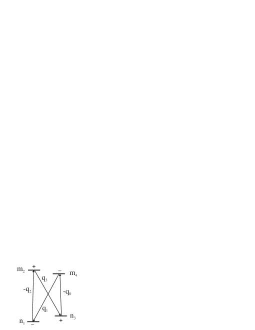
Figure 4: Four-level diagram corresponding to resonance scattering of light.

[it is necessary to associate a oriented line segment $\overset{q_{k}}{\longrightarrow}$ from $m_{i}$-(sub)level to $n_{j}$-(sub)level with $T^{m_{i}n_{j}}_{\dot{q}{}_{k}}$]. In cases $J_{mn}=\pm 1$, in accordance with selection rules [see (40) and further between (80) and (81)], the spectral manifestations of four-level diagrams with unequal (both lower and upper) indices are essentially weakened. The situation is better, when there is index coincidence only in one pair of lower or upper levels, that gives the Raman three-level diagrams, respectively, $\bm{\vee}$- or $\bm{\wedge}$-types. Their spectral manifestations, as “Raman HFS” of the same types, are conditioned by appropriate complex resonance co-factor from the pair disposed in denominator of expression (65b) (the complexity can be manifested only in the diagrams with differently polarized light components). At last the simultaneous index coincidences in both upper and lower level pairs give the two-level diagrams of $\bm{\between}$-types. The collision constants then enter only in a simple nonresonance factor $\nu^{2}/\nu_{m}\nu_{n}$, and all resonance feature are determined with field dependence of real numerator of expression (65b). We have introduced the name “ballast HFS” for resonance structures of the last type. In the pure state they are present in the transmission of circularly polarized radiation. Their distinctive feature is always negative sign with respect to Raman HFS. It is possible to make certain of it, e.g., using just described expansion of expression (65b) on components: $\bm{\between}+\bm{\vee}+\bm{\wedge}+{\Join}$. It is easy to see, that all the components, except last one, are positive. For transitions with changing $J_{j}$, the last one can be rejected, as it has the next smallness order $J^{-4}$ with respect to previous components; when $B^{(0)}=0$, it is visible from (40). As a result, using an inequality

$$\left|\mathop{\mathrm{Re}}\prod_{j}(1-\mathrm{i}x_{j})^{-1}\right|\leq 1$$

with $x_{j}\in\mathbb{R}$, we have

$$\bm{\between}+\bm{\vee}+\bm{\wedge}+{\Join}\leq\text{wing},$$ (66)

i.e., if the radiation is circularly polarized, the total expression (65b) with any $B^{(0)}$ near resonance, is always less than its wing value, when $B^{(0)}$ is large. The first summand in (66) is always resonance. The residuals are completely or partially suppressed (in according to whether $\nu=0$ or not) because of their nonresonance character connected to anti-crossings of the diagram levels. With large $\nu$ all four summands in sum (66) reproduce the wing.

For multi-spin molecule the resonance for circularly polarized radiation consists of several dips. These dips are manifested, when light interacts with rotation subsystem and feels that the hyperfine coupling of any spin subsystem (as a ballast) take place. Thus, unlike Raman scattering, the gas medium property to absorb light is increased. The light energy indirectly comes in nuclear spin subsystems and is spent on flipping nuclear spins of molecule.

An elementary mechanical model, imitating the ballast structure of the spectrum, consists of two interacting tops. E.g., let they will be a pencil vertically clamped in hands and a gramophone plate freely pined upon it. The pencil here corresponds to rotation subsystem and the plate — to ballast spin one. The small friction between them corresponds to hyperfine coupling (without precession). Twisting the pencil between hands we shall imitate an influence of light to our molecule being capable of its absorption. The frequency of twisting is analog of a collision frequency $\nu$, restricting the influence of light. Comparing these absorption capabilities determined with the low and high frequencies, it is not difficult to see that it is higher in the first case than in the second one. In the first case the pencil and the plate rotate together as a whole. In the second case the pencil rotates, practically not having time to pull about the pined plate.

In other (equivalent) interpretation the ballast structure — the manifestation of anti-crossings of hyperfine magnetic sublevels [5]. For the first time this structure was observed in resonance fluorescence of lithium atoms [4]. As it is known [9], the structure of field spectra in nonlinear transmission of pumping (47) is analogous to the structure in resonance fluorescence [3]

$$s^{(2)}_{(\bm{e},\bm{f})}=\tilde{\bm{X}}{}^{(3)mn}_{(\hat{H}^{(1)}_{n}=0)}\,\underset{\displaystyle\cdot}{\vdots}\,\bm{f}^{*}\otimes\bm{e}\otimes\bm{e}^{*}\otimes\bm{f}\quad(\in\mathbb{R}).$$ (67)

Here nonlinear cubic susceptibility (55) or differently fourth rank tensor (50) of gas medium is contracted twice with $\bm{e}$ and twice with $\bm{f}$, respectively, the unit polarization vectors of optical pumping (excitation) and resonance fluorescence; also it is noted, that the multiplet structure of lower level ($n$) in resonance fluorescence of upper one ($m$) is not manifested (and that ensures the real value of contracted expression). However, the analogy and comparison are possible only theoretically, as both ordinary and resonance fluorescences in our IR range are practically unobservable, unlike nonlinear transmission of pumping.

As an example to the described classification we shall represent the results of exact calculations of formula (65b) with use of a computer, for NOR/M_∥ in radiation transmission of methane isotope ${}^{12}\mathrm{CH}_{4}$. In Figure 5, concerning to a linearly polarized radiation, the Raman HFS is shown obviously with impurity of ballast.

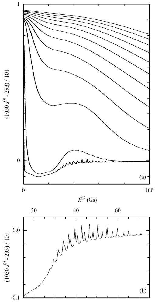
Figure 5: Exact calculated NOR/M_∥ (even functions) in transmission of linearly polarized radiation for component ($\omega_{3}$ $P(7)$ $F^{(2)}_{2(-)}$) of isotope ${}^{12}\mathrm{CH}_{4}$: (a) $\nu=0.1$, $1$, $10$, $20$, $\ldots$, $100\,\mathrm{kHza}$ (the curves with greater $\nu$ pass higher); (b) $\nu=0.1\,\mathrm{kHza}$.

The purely Raman HFS consists of peaks only and never passes below than wing level at large $B^{(0)}$. The purely ballast HFS is shown in next Figure 6, concerning to circularly polarized radiation.

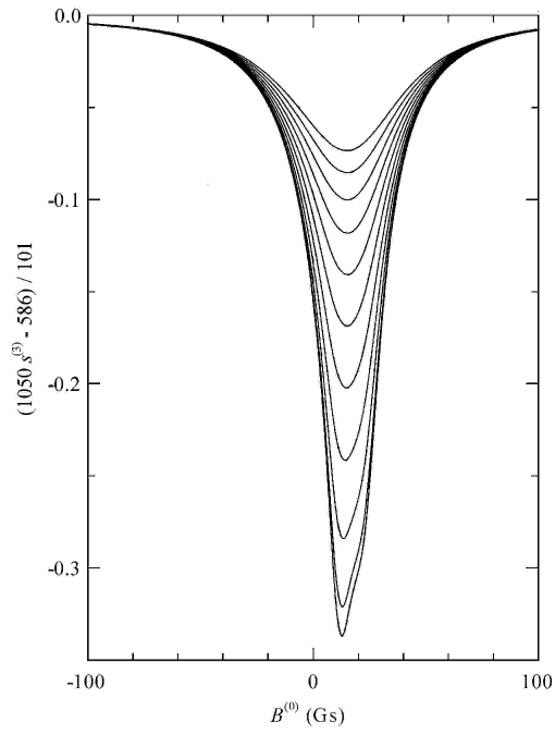
Figure 6: Exactly calculated NOR/M_∥ in transmission of right circularly polarized radiation for component ($\omega_{3}$ $P(7)$ $F^{(2)}_{2(-)}$) of isotope ${}^{12}\mathrm{CH}_{4}$: $\nu=0.1$, $1$, $10$, $20$, $\ldots$, $100\,\mathrm{kHza}$ (the dip with maximal depth practically corresponds to the first two cases, and the ones with greater $\nu$ are shallower).

It is practically symmetric dip, displaced to the right for rightly polarized radiation. The dip for contrary polarized radiation is obtained by mirror reflection with respect to ordinate axis, i.e. its shift has opposite sign. The shift does not practically depend on pressure. With increasing $\nu$ on an order, from $10$ to $100\,\mathrm{kHza}$, the width on half-depth and the depth of the dip are approximately doubled and quartered, respectively.

To facilitate a comparison with the above-represented experimental data, derivatives are shown in Figure 7, and they appropriate to the previous two FIGs.

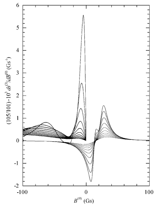
Figure 7: Derivatives of exact calculated NOR/M_∥ in transmission of radiations polarized linearly (odd functions; their negative branches with $B^{(0)}>0$ are omitted) and right-circularly for component ($\omega_{3}$ $P(7)$ $F^{(2)}_{2(-)}$) of isotope ${}^{12}\mathrm{CH}_{4}$: $\nu=10,20,\ldots,100\,\mathrm{kHza}$ (here the curves with greater $\nu$ have smaller amplitude).

Judging by amplitude ratio of narrow and wide structures for linearly polarized radiation, the experimental curves in Figure 2 at the left correspond to case $\nu\simeq 40\,\mathrm{kHza}$. As we have seen, the dip in Figure 6 for circularly polarized radiation is practically symmetric and displaced. Respectively, the dip derivative is antisymmetric and also displaced. For the more detailed analysis it is convenient to describe an existing small quantity of dip asymmetry for circularly polarized radiation in the following way. On a curve, representing derivative, let us mark (always existing) two ordered points, where the module of amplitude of this derivative is maximum, by means of coordinates $(B^{(0)},\partial s^{(3)}/\partial B^{(0)})$, namely, $(x_{0},y_{0})$ and $(x_{1},y_{1})$. An ordering condition for the points is $|x_{0}|<|x_{1}|$. It is convenient for that allows to do not pay attention to what circular polarization is considered. The quantity of dip asymmetry is now determined as $a_{y}=1-|y_{0}/y_{1}|$. Judging by Figure 7, this quantity is small and also changes its sign at $\nu\simeq 30\,\mathrm{kHza}$. There is a feature observed in Figure 7 only with small $\nu$, when the second field derivative in the area of resonance (without wings) begins to have four zero points instead of two ones. It is possible to estimate the position of the feature, changing the asymmetry sign, as (28). It is approximately greater by factor of $\sqrt{2}$ than the dip shift or otherwise the position of its lower point, see below (88).

The described structures can be represented in zero-pressure limit, when $\nu$ is determined only by spontaneous decay. In Figure 5(b) at nonzero fields we clearly distinguish the two types of peaks grouped in pairs, $\bm{\vee}^{m\prime}_{nq}$ and $\bm{\wedge}^{m\prime}_{nq}$. Without HFS, according to (2c), the amplitude ratio of peaks at zero field is $\bm{\vee}^{m\prime}_{nq}/\bm{\wedge}^{m\prime}_{nq}\simeq a^{2}_{m2}/a^{2}_{n2}$ and $\lesseqqgtr 1$, if $J_{mn}\lesseqqgtr 0$, respectively. With HFS, there is the similar amplitude ratio of peaks at nonzero fields. We mention in passing that the approximation, represented in the next section 4, is not sufficient for real deriving of this ratio.

In appendix the classification, represented here for HFS of NOR/M, understands on a simple model case, when both level angular momenta and spin are equal $1/2$. Let us note, that the case does not concern directly to the molecules considered by us, and what is more the case does not concern also to atoms. In their visible frequency area, instead of HFS an other structure goes out on the first plan, namely, spontaneous one, connected with the induced two-photon absorption through an intermediate spontaneous decay [22].

Coming back to the formulae (65), we shall note the following. Here we use only the expression (65b), but the initial expression (65a) can be invariantly calculated, i.e. without the help of specific basis of wave functions. Properly using only commutation relations for tensor components of operators included in it, at first the trace $\langle\ldots\rangle$ may be calculated, and then time integrals. Another alternative calculation way is possible also, permitting to interchange the sequence of these operations. For that it is necessary to use a resolvent representation of evolutionary operators [1, Chap. XXI § 13] (see also [29, Chap. V § 4]):

$$\mathop{\mathrm{e}}\nolimits^{\bar{\mathrm{i}}\hat{H}^{(1)}_{j}t}=\oint\limits_{\circlearrowleft}\frac{\mathrm{d}z}{2\pi\mathrm{i}}\mathop{\mathrm{e}}\nolimits^{\bar{\mathrm{i}}zt}\hat{R}^{(1)}_{j}(z).$$ (68)

The resolvent $\hat{R}^{(1)}_{j}(z)$ has defined in (19). Its complex spectral parameter $z$ passes on integration contour $\circlearrowleft$, enveloping all points of spectrum for operator $\hat{H}^{(1)}_{j}$, i.e.  the poles (singularities) of its resolvent. After calculation in (65a) the time integrals, we obtain

$$X^{(3)mn}_{\underset{\scriptstyle\dot{}}{q}{}_{0}\dot{q}{}_{1}\underset{\scriptstyle\dot{}}{q}{}_{2}\dot{q}{}_{3}}(B^{(0)})=\mathop{\mathrm{e}}\nolimits^{-(\varOmega_{q_{2}}/\omega_{\mathrm{D}})^{2}}\left(\prod_{k=1,2,3,4}\oint\limits_{\circlearrowleft}\frac{\mathrm{d}z_{k}}{2\pi\mathrm{i}}\right)\frac{\nu^{2}}{(\nu_{m}-\mathrm{i}z_{24})(\nu_{n}-\mathrm{i}z_{31})}\\ \times\left\langle\hat{T}^{mn\dagger}_{\dot{q}{}_{0}}\hat{R}^{(1)}_{m}(z_{4})\hat{T}^{mn}_{\dot{q}{}_{1}}\hat{R}^{(1)}_{n}(z_{1})\hat{T}^{mn\dagger}_{\dot{q}{}_{2}}\hat{R}^{(1)}_{m}(z_{2})\hat{T}^{mn}_{\dot{q}{}_{3}}\hat{R}^{(1)}_{n}(z_{3})\right\rangle$$ (69)

From here at once, using the basis (21a), the equation (65b) is obtained. However it is possible to calculate the expression (69), as well as (65a), without concretizing the basis set of wave functions. In the given paper we shall not go into more details of these two ways of calculation.

The model, used by us, has simple and rather reliable basis in itself. What concerns a comparison with methane experiment, here a discussion can go only about details. E.g., if someone will interest collision components, their calculation in the model of strong deorientational collisions is produced below in section 5. One may assume that the transition to other molecules is more actual. The main (hyperfine) structure of the field spectrum of NOR will be thus involved. E.g., in section 6 the molecule of fluoromethane is considered.

4 High-$J$ approximation of HFS of NOR/M_∥ in ${}^{13}\mathrm{CH}_{4}$

To simplify the analysis of the problem, when spin subsystems more than one, we consider the states, in which the molecule rotates rather fast. Owing to that, in (22) one can take into consideration only isotropic (scalar) spin-rotation interaction, as in (10). When $J\gg I^{\varsigma}$ for all $\varsigma$, it is possible to put down in (16) for zero approximation

$$\bm{J}_{j,M-\underline{\hat{I}}{}_{z}}\simeq\bm{J}_{jM}\simeq\left(\sqrt{\hat{\bm{J}}{}_{j}^{2}-M^{2}},0,M\right)_{x,y,z}.$$ (70)

In the last expression we used that $J_{y,jM}\simeq 0$. Thus we obtain a linearization of Hamiltonian (16) on spins $\underline{\hat{\bm{I}}}{}^{\varsigma}$, i.e.

$$\underline{\hat{h}}{}^{\varsigma}_{jM}\simeq-\left(C^{\varsigma}_{\mathrm{a}}\bm{J}^{*}_{jM}+\bm{\varDelta}^{\varsigma}_{IJ}\right)\cdot\underline{\hat{\bm{I}}}{}^{\varsigma}\simeq-\bm{\omega}^{\varsigma}_{jM}\cdot\underline{\hat{\bm{I}}}{}^{\varsigma},$$ (71a)

where vector

$$\bm{\omega}^{\varsigma}_{jM}\simeq\left(C^{\varsigma}_{\mathrm{a}}\sqrt{\hat{\bm{J}}{}_{j}^{2}-M^{2}},0,C^{\varsigma}_{\mathrm{a}}M+\varDelta^{\varsigma}_{IJ}\right)_{x,y,z}.$$ (71b)

In this approximation the commutator $[\underline{\hat{h}}{}^{\varsigma_{1}}_{jM_{1}},\underline{\hat{h}}{}^{\varsigma_{2}}_{jM_{2}}]=0$, therefore it is possible to consider independently all interactions of rotation subsystem with spin ones. We shall use approximately factored transforming operators in (21a), namely

$$\hat{\mathcal{U}}_{jM}\simeq\prod_{\varsigma}\hat{\mathcal{U}}{}^{\varsigma}_{jM}\simeq\prod_{\varsigma}\mathop{\mathrm{e}}\nolimits^{\bar{\mathrm{i}}\beta^{\varsigma}_{jM}\hat{I}^{\varsigma}_{y}}$$ (72)

with $\hat{I}{}^{\varsigma}_{y}=\bm{u}^{\varsigma}_{y}\cdot\hat{\bm{I}}{}^{\varsigma}$. Now this transformation is the set of independent rotations in spin function spaces around basis vectors $\bm{u}^{\varsigma}_{y}$ on angles $\beta^{\varsigma}_{jM}$, which are determined through unit vectors

$$\left(\sin\beta^{\varsigma}_{jM},0,\cos\beta^{\varsigma}_{jM}\right)_{x,y,z}=\bm{n}^{\varsigma}_{jM}\equiv\bm{\omega}^{\varsigma}_{jM}/\omega^{\varsigma}_{jM}.$$ (73)

The rotation is arranged so, that all matrices $\underline{\hat{h}}{}^{\varsigma}_{jM}$ in (16), originally defined by us in old basis (15a), will be transformed in unitarily similar diagonal ones $\underline{\hat{h}}{}^{\varsigma\prime}_{jM}$, defined in new basis (21a), i.e.

$$\left(\underline{\hat{h}}{}^{\prime}_{jM}\right)_{\tilde{\mu}^{\bm{\cdot}}\tilde{\mu}^{\bm{\cdot}}}=\langle j\tilde{\mu}^{\bm{\cdot}}M|\hat{h}_{j}|j\tilde{\mu}^{\bm{\cdot}}M\rangle$$

and

$$\underline{\hat{h}}{}^{\prime}_{jM}=\hat{\mathcal{U}}^{\dagger}_{jM}\underline{\hat{h}}{}_{jM}\hat{\mathcal{U}}_{jM}=-\sum_{\varsigma}\omega^{\varsigma}_{jM}\underline{\hat{I}}{}^{\varsigma}_{z}.$$ (74)

Thus the (hyperbolic) approximation of spectrum of total Hamiltonian is

$$H^{(1)}_{j\tilde{\mu}^{\bm{\cdot}}_{j}M}=-\sum_{\varsigma}\tilde{\mu}^{\varsigma}_{j}\omega^{\varsigma}_{jM}-\varDelta_{J}M.$$ (75)

The expansion near $B^{(0)}=0$ is

$$H^{(1)}_{j\tilde{\mu}^{\bm{\cdot}}_{j}M}(B^{(0)})\simeq-\sum_{\varsigma}\tilde{\mu}^{\varsigma}_{j}C^{\varsigma}_{\mathrm{a}}(J_{j}+1/2)-M\gamma^{(\mathrm{eff})}_{j\tilde{\mu}^{\bm{\cdot}}_{j}}B^{(0)}.$$ (76a)

Effective gyromagnetic ratio

$$\gamma^{(\mathrm{eff})}_{j\tilde{\mu}^{\bm{\cdot}}_{j}}=\left.\gamma^{(\mathrm{eff})}_{j\tilde{\mu}^{\bm{\cdot}}_{j}M}\right|_{B^{(0)}=0}=\left.-M^{-1}\partial_{B^{(0)}}H^{(1)}_{j\tilde{\mu}^{\bm{\cdot}}_{j}M}\right|_{B^{(0)}=0}\simeq\gamma_{J}+\sum_{\varsigma}\tilde{\mu}^{\varsigma}_{j}\gamma^{\varsigma}_{IJ}/(J_{j}+1/2),$$ (76b)

where there is summation on spin subsystems $\varsigma$ with $C^{\varsigma}_{\mathrm{a}}\neq 0$ only. From here one can determine the total ordered set of $g$-factors, $g^{(\mathrm{eff})}_{j\tilde{\mu}^{\mathrm{H}}}=\gamma^{(\mathrm{eff})}_{j\tilde{\mu}^{\mathrm{H}}}/\gamma_{\mathrm{N}}$, for $P(7)$-branch of methane with $I^{\mathrm{H}}=1$:

$$\begin{split}g^{(\mathrm{eff})}_{m;\bar{1},0,1}&\simeq-0.5,\,0.3,\,1.1\\ \text{and}\quad g^{(\mathrm{eff})}_{n;\bar{1},0,1}&\simeq-0.4,\,0.3,\,1.\end{split}$$ (77)

The exact expressions for $g$-factors (24) can be compared with their approximation (76b) in the form of gyromagnetic ratios.

In split basis of wave functions (15a), the matrix elements of covariant components of standard vectorial operator of ${[}^{m}_{n}$-transition are

$$\left(\underline{\hat{T}}{}^{mn}_{\dot{q}{}M}\right)_{\mu^{\bm{\cdot}}\mu^{\bm{\cdot}}}\equiv\langle m\mu^{\bm{\cdot}}M+q|\hat{T}^{mn}_{\dot{q}{}}|n\mu^{\bm{\cdot}}M\rangle$$

with

$$\underline{\hat{T}}{}^{mn}_{\dot{q}{}M}=T^{mn}_{\dot{q}{}(M-\underline{\hat{I}}{}_{z})}.$$ (78a)

In new basis (21a)

$$\left(\underline{\hat{T}}{}^{mn\prime}_{\dot{q}{}M}\right)_{\tilde{\mu}^{\bm{\cdot}}_{m}\tilde{\mu}^{\bm{\cdot}}_{n}}\equiv\langle m\tilde{\mu}^{\bm{\cdot}}_{m}M+q|\hat{T}^{mn}_{\dot{q}{}}|n\tilde{\mu}^{\bm{\cdot}}_{n}M\rangle$$

with

$$\underline{\hat{T}}{}^{mn\prime}_{\dot{q}{}M}=\hat{\mathcal{U}}^{\dagger}_{m,M+q}\underline{\hat{T}}{}^{mn}_{\dot{q}{}M}\hat{\mathcal{U}}_{nM}\simeq\mathop{\mathrm{e}}\nolimits^{\mathrm{i}\sum_{\varsigma}\beta^{\varsigma mn}_{qM}\underline{\hat{I}}{}^{\varsigma}_{y}}T^{mn}_{\dot{q}{}\bigl{(}M-\sum_{\varsigma}(n^{\varsigma}_{z,nM}\underline{\hat{I}}{}^{\varsigma}_{z}-n^{\varsigma}_{x,nM}\underline{\hat{I}}{}^{\varsigma}_{x})\bigr{)}}$$ (78b)

Using here the Taylor expansion on $$\underline{\hat{\bm{I}}}{}^{\varsigma}$$ and being limited quadratic summands, we obtain

$$\underline{\hat{T}}{}^{mn\prime}_{\dot{q}{}M}\Rightarrow T^{mn}_{\dot{q}{}M}\left\{\hat{1}-\sum_{\varsigma}\left[\frac{\partial_{M}T^{mn}_{\dot{q}{}M}}{T^{mn}_{\dot{q}{}M}}n^{\varsigma}_{z,nM}\underline{\hat{I}}{}^{\varsigma}_{z}+\frac{1}{\sqrt{2}}\left(\beta^{\varsigma mn}_{qM}+\frac{\partial_{M}T^{mn}_{\dot{q}{}M}}{T^{mn}_{\dot{q}{}M}}n^{\varsigma}_{x,nM}\right)\underline{\hat{I}}{}^{\varsigma}_{\dot{1}}\right.\right.\\ \left.\left.+\frac{1}{\sqrt{2}}\left(\beta^{\varsigma mn}_{qM}-\frac{\partial_{M}T^{mn}_{\dot{q}{}M}}{T^{mn}_{\dot{q}{}M}}n^{\varsigma}_{x,nM}\right)\underline{\hat{I}}{}^{\varsigma}_{\dot{\bar{1}}}+\frac{1}{2}\beta^{\varsigma mn2}_{qM}\underline{\hat{I}}{}^{\varsigma 2}_{y}\right]\right\}.$$ (78c)

The arrow ($\Rightarrow$) here marks that from quadratic corrections only one is kept, which gives the contribution to resonance.

Here the covariant spherical components $\underline{\hat{I}}{}^{\varsigma}_{\dot{q}}$ are standardly defined and similar with (14). The difference $\beta^{\varsigma mn}_{qM}\equiv\beta^{\varsigma}_{m,M+q}-\beta^{\varsigma}_{nM}$ and small, therefore below, in (86), it is possible to substitute

$$\beta^{\varsigma mn}_{qM}\simeq\sin\beta^{\varsigma mn}_{qM}=-[\bm{n}^{\varsigma}_{m,M+q}\times\bm{n}^{\varsigma}_{nM}]_{y}.$$ (79)

As it was above noted, when the field $B^{(0)}$ is close to zero, $F^{\varsigma}_{j}-J_{j}\simeq\tilde{\mu}^{\varsigma}_{j}$, where $\hat{\bm{F}}{}^{\varsigma}_{j}=\hat{\bm{J}}_{j}+\hat{\bm{I}}{}^{\varsigma}$. Here there are selection rules for the matrix elements of electro-dipole transition ${[}^{m}_{n}$ [42], namely,

$$|F^{\varsigma}_{mn}|=|J_{mn}+\tilde{\mu}^{\varsigma}_{mn}|\leq 1$$ (80)

with $\tilde{\mu}^{\varsigma}_{mn}\equiv\tilde{\mu}^{\varsigma}_{m}-\tilde{\mu}^{\varsigma}_{n}$, also $F^{\varsigma}_{m}+F^{\varsigma}_{n}\geq 1$ and for parities $p_{m}p_{n}=-1$.

When the field $B^{(0)}$ is arbitrary, we can use the expansion (78c). The corrections, giving the contributions only in resonance wing, have been omitted though they are important for selection rules of weaker (satellite) transitions. The given expansion gives us selection rules in arbitrary magnetic field, when there are the main transitions with an order $\epsilon\equiv|\tilde{\mu}^{\varsigma}_{mn}|=0$ and satellite ones with $\epsilon=1,2,\ldots$. The satellite transitions are weaker, $\propto J^{-\epsilon}$, in respect to main ones. Let us remark, that in the correspondence with (80) for $J_{mn}=-1$, i.e.  in $P$-branch, there should be an asymmetry of satellites [see also (40)]. Projecting it on (78c), we see that in the first order at satellites it should be

$$\left(\beta^{\varsigma mn}_{qM}-\frac{\partial_{M}T^{mn}_{\dot{q}{}M}}{T^{mn}_{\dot{q}{}M}}n^{\varsigma}_{x,nM}\right)_{B^{(0)}=0}=0$$ (81)

and similarly in the second one (of course taking into account the dropped wing corrections). At $B^{(0)}=0$, according to (80), in $P$-branch the satellites with more than second order should not be at all. Within the framework of our approximation it is applied not for all $M$, though the tendency to that is kept and conducts to partial suppression of $\Join$-type summands for NOR/M_∥ in $P$-branch.

To describe structural features of NOR/M_∥ in linearly polarized radiation, it is enough to take into account the fixed contribution of main transitions in Taylor expansion for (78c) with $|\tilde{\mu}^{\varsigma}_{mn}|=0$ and even without the contributions $\sim J^{-1}$ with respect to fixed one. As a result we obtain

$$\bm{\vee}^{m}_{nq}+\bm{\wedge}^{m}_{nq}\equiv X^{(3)mn}_{\underset{\scriptstyle\dot{}}{q}{}\dot{q}{}\underset{\scriptstyle\dot{}}{\bar{q}}{}\dot{\bar{q}}{}}+X^{(3)mn}_{\underset{\scriptstyle\dot{}}{q}{}\dot{\bar{q}}{}\underset{\scriptstyle\dot{}}{\bar{q}}{}\dot{q}{}}$$

$$\simeq\mathop{\mathrm{e}}\nolimits^{-(\varOmega_{\bar{q}}/\omega_{\mathrm{D}})^{2}}\frac{\nu^{2}}{\nu_{m}\nu_{n}}\sum_{\tilde{\mu}^{\bm{\cdot}}M}\left[\frac{|T^{mn}_{\dot{q}{}M}T^{mn}_{\dot{\bar{q}}{}M}|^{2}\,\nu_{m}}{\nu_{m}-\mathrm{i}\left(2q\varDelta_{J}+\sum_{\varsigma}\tilde{\mu}^{\varsigma}\omega^{\varsigma mm}_{M+q,M-q}\right)}+(m\leftrightarrow n)\right].$$ (82)

Here $\omega^{\varsigma j^{\prime}j}_{M^{\prime}M}\equiv\omega^{\varsigma}_{j^{\prime}M^{\prime}}-\omega^{\varsigma}_{jM}$. The summands in square brackets of the formula are ordered and obtained by mutual permutation of indices, i.e. $\bm{\wedge}^{m}_{nq}=\bm{\vee}^{n}_{mq}$ (however $\omega_{mn}$ in $\varOmega_{\bar{q}}$ by this permutation is not affected). The formula describes a set of peaks of Raman scattering of $\bm{\vee}$- and $\bm{\wedge}$-types at crossings of hyperfine magnetic sublevels, therefore we have named this structure of NOR/M as Raman one. Because of complexity it can be found out with both amplitude and phase measurements. The complexity is connected with polarization opposition of photons, forming a combining pair in scattering. It is visible, that $\bm{\vee}^{m*}_{nq}=\bm{\vee}^{m}_{n\bar{q}}$ and $\bm{\wedge}^{m*}_{nq}=\bm{\wedge}^{m}_{n\bar{q}}$. The condition of manifestation of Raman HFS of NOR/M in nonzero fields by means of a set of peaks is $\nu\leq|C^{\varsigma}_{\mathrm{a}}|$. Especially it is necessary to draw attention to zero peak, when $\nu\gg|C^{\varsigma}_{\mathrm{a}}|$. It continues to look as a cusp on the background of collision Raman non-hyperfine NOR/M, if the degree of its quadratic sharpness with respect to the background is ratio

$$\frac{\partial^{2}_{B^{(0)}}\left[\bm{\vee}^{m\prime}_{n,1}+\bm{\wedge}^{m\prime}_{n,1}\right]^{(\text{all }C^{\varsigma}_{\mathrm{a}}\neq 0)}_{B^{(0)}=0}}{\partial^{2}_{B^{(0)}}\left[\bm{\vee}^{m\prime}_{n,1}+\bm{\wedge}^{m\prime}_{n,1}\right]^{(\text{all }C^{\varsigma}_{\mathrm{a}}=0)}_{B^{(0)}=0}}\simeq(\prod_{\varsigma}[I^{\varsigma}])^{-1}\sum_{j\tilde{\mu}^{\bm{\cdot}}}g^{(\mathrm{eff})2}_{j\tilde{\mu}^{\bm{\cdot}}}/2g^{2}_{J}>1,$$ (83)

where effective $g$-factors (or respective gyromagnetic ratios $\gamma$) and the condition of summation on spin subsystems $\varsigma$ are the same with (76b). For methane, when $P(7)$-branch is considered and $I=1$, the ratio $\simeq 5$. Thus, if collision Raman non-hyperfine NOR/M is observed, then its sub-collision HFS is observed all the more. The structure in the pure kind is inconvenient for observation in transmission, and convenient in birefringence, as it was made in [20]. There was registration of field derivative of rotation angle of light polarization plane. In conditions, when saturation parameter $\varkappa\gg\nu/\omega_{\mathrm{D}}$, the angle

$$\theta\simeq\theta^{(3)}\propto\bm{\vee}^{m\prime\prime}_{n,1}+\bm{\wedge}^{m\prime\prime}_{n,1}.$$ (84)

The sub-collision Raman HFS (without ballast one) was observed on background of Raman non-hyperfine one as a cusp of $\partial_{B^{(0)}}\theta$. The degree of its sharpness can be found from ratio

$$\frac{\partial^{3}_{B^{(0)}}\left[\bm{\vee}^{m\prime\prime}_{n,1}+\bm{\wedge}^{m\prime\prime}_{n,1}\right]^{(\text{all }C^{\varsigma}_{\mathrm{a}}\neq 0)}_{B^{(0)}=0}}{\partial^{3}_{B^{(0)}}\left[\bm{\vee}^{m\prime\prime}_{n,1}+\bm{\wedge}^{m\prime\prime}_{n,1}\right]^{(\text{all }C^{\varsigma}_{\mathrm{a}}=0)}_{B^{(0)}=0}}\simeq(\prod_{\varsigma}[I^{\varsigma}])^{-1}\sum_{j\tilde{\mu}^{\bm{\cdot}}}g^{(\mathrm{eff})3}_{j\tilde{\mu}^{\bm{\cdot}}}/2g^{3}_{J}>1,$$ (85)

and for methane ($P(7)$-branch and $I=1$) the ratio $\simeq 14$. If we judge by the signal approximation (82), there is just its cusp, (83) or (85), in field zero, but its amplitude here does not vary. The signal amplitude in Figure 5 is mainly varied through both $\bm{\between}$-type summands in (48).

Thus, after passage by linearly polarized radiation of absorbing cell, its field spectrum acquires components, which look as peaks in amplitude measurements. They are conditioned by process of resonance scattering with crossings of hyperfine sublevels in magnetic field, when $[2q\varDelta_{J}+\sum_{\varsigma}\tilde{\mu}^{\varsigma}\omega^{\varsigma jj}_{M+q,M-q}]=0$ with $j\in(m,n)$. The greatest amplitude has peak at field zero, due to large number of sublevel crossings. Peaks are grouped in area of nonzero fields, where (27), from single crossings in sublevel pairs with $|M^{\prime}_{j}-M_{j}|=2$ and $\tilde{\mu}^{\mathrm{H}\prime}_{j}=\tilde{\mu}^{\mathrm{H}}_{j}=-1$. For ${}^{12}\mathrm{CH}_{4}$ with rather low pressure there are only two such areas located mutually symmetrically from field zero. For ${}^{13}\mathrm{CH}_{4}$ with similar pressure these areas of crossings are split on pairs ($\tilde{\mu}^{\mathrm{H}},\tilde{\mu}^{\mathrm{C}}$); in the beginning ($-1,-\frac{1}{2}$) and further ($-1,\frac{1}{2}$), if we scan from field zero (appropriate FIGs. are omitted). The half-width of these peaks is determined by magnitude $\nu/2\gamma$ with slightly distinguishing $\gamma$-factors varying near $\gamma_{J}$. If we direct $\nu$ to zero, when magnetic field is non-peak, we shall receive $(\bm{\vee}^{m}_{nq}+\bm{\wedge}^{m}_{nq})\rightarrow 0$. This property is unconnected with the approximation, used in (82), and kept in exact calculation. In Figure 5, i.e. in amplitude measurements (48), the Raman peaks is observed on the background of both ballast dips. In any way the resonance curve below than wing level could not be lowered without theirs. As we have already noted, the last ones disappear in phase measurements. When $\nu\gg|C^{\varsigma}_{\mathrm{a}}|$ for all $\varsigma$, the Raman structure of NOR/M smooths out and we see single (practically Lorentz) contour with half-width $\nu/2\gamma_{J}$ (see Figure 1). Its top is nevertheless sharpened, according to (83). Because of its small amplitude it is better to observe the cusp in the field derivatives of transmission, as in Figure 7, or circular birefringence (84), as in [20].

Without hyperfine interaction for NOR/M in linearly polarized radiation there is a frequency analog [see (2c)], i.e. $\varDelta_{J}\leftrightarrow\omega_{\varDelta}$, and also analog of Kramers-Kronig relation for amplitude and phase [43]. HFS breaks this relation and that also can be used for extracting of its contribution in linearly polarized radiation.

To describe field structures of NOR/M_∥ in circularly polarized radiation it is necessary to expand (78b) in a series (78c), i.e., in addition to main transitions with $|\tilde{\mu}^{\varsigma}_{mn}|=0$, to take into account weaker satellite ones with $|\tilde{\mu}^{\varsigma}_{mn}|=1,2$. The magnetic and hyperfine properties of both $j$-terms are close among themselves, therefore $|\beta^{\varsigma mn}_{qM}|\ll 1$ and it is possible to use (79). Taking into account all that, we obtain

$$\bm{\between}^{m}_{nq}\equiv X^{(3)mn}_{\underset{\scriptstyle\dot{}}{q}{}\dot{q}{}\underset{\scriptstyle\dot{}}{q}{}\dot{q}{}}\simeq\mathop{\mathrm{e}}\nolimits^{-(\varOmega_{q}/\omega_{\mathrm{D}})^{2}}\frac{\nu^{2}}{\nu_{m}\nu_{n}}\prod_{\varsigma^{\prime}}[I^{\varsigma^{\prime}}]\sum_{M}|T^{mn}_{\dot{q}{}M}|^{4}\left\{1-\frac{2}{3}\sum_{\varsigma}\hat{\bm{I}}{}^{\varsigma 2}\vphantom{\left(\frac{\partial_{M}T^{mn}_{\dot{q}{}M}}{T^{mn}_{\dot{q}{}M}}n^{\varsigma}_{x,nM}\right)^{2}}\right.$$

$$\times\left[(\bm{n}^{\varsigma}_{m,M+q}\times\bm{n}^{\varsigma}_{nM})^{2}+3\left(\frac{\partial_{M}T^{mn}_{\dot{q}{}M}}{T^{mn}_{\dot{q}{}M}}n^{\varsigma}_{x,nM}\right)^{2}\right.$$ (86a)

$$-\left((\bm{n}^{\varsigma}_{m,M+q}\times\bm{n}^{\varsigma}_{nM})^{2}+\left(\frac{\partial_{M}T^{mn}_{\dot{q}{}M}}{T^{mn}_{\dot{q}{}M}}n^{\varsigma}_{x,nM}\right)^{2}\right)\left(\frac{\nu_{m}^{2}}{\nu_{m}^{2}+\omega^{\varsigma 2}_{m,M+q}}+\frac{\nu_{n}^{2}}{\nu_{n}^{2}+\omega^{\varsigma 2}_{n,M}}\right)$$ (86b)

$$\left.\left.+\left((\bm{n}^{\varsigma}_{m,M+q}\times\bm{n}^{\varsigma}_{nM})^{2}-\left(\frac{\partial_{M}T^{mn}_{\dot{q}{}M}}{T^{mn}_{\dot{q}{}M}}n^{\varsigma}_{x,nM}\right)^{2}\right)\frac{\nu_{m}^{2}\,\nu_{m}^{2}}{(\nu_{m}^{2}+\omega^{\varsigma 2}_{m,M+q})(\nu_{n}^{2}+\omega^{\varsigma 2}_{n,M})}\right]\right\}$$ (86c)

$$\simeq\mathop{\mathrm{e}}\nolimits^{-(\varOmega_{q}/\omega_{\mathrm{D}})^{2}}\prod_{\varsigma^{\prime}}[I^{\varsigma^{\prime}}]\sum_{M}|T^{mn}_{\dot{q}{}M}|^{4}\left\{1-\frac{2}{3}\sum_{\varsigma}\hat{\bm{I}}{}^{\varsigma 2}\right.$$

$$\times\left.\left[\frac{(\bm{\omega}^{\varsigma}_{m,M+q}\times\bm{\omega}^{\varsigma}_{nM})^{2}}{(\nu^{2}+\omega^{\varsigma 2}_{m,M+q})(\nu^{2}+\omega^{\varsigma 2}_{nM})}+\left(\frac{\partial_{M}T^{mn}_{\dot{q}{}M}}{T^{mn}_{\dot{q}{}M}}\right)^{2}\left(3+\frac{\nu^{2}}{\nu^{2}+\omega^{\varsigma 2}_{nM}}\right)\frac{\omega^{\varsigma 2}_{x,nM}}{\nu^{2}+\omega^{\varsigma 2}_{nM}}\right]\right\}.$$ (86d)

The unit vectors $\bm{n}^{\varsigma}_{jM}$ are defined in (73). At first, in (square) brackets, we have disjointed the structures of $\bm{\between}$-type (86a), $(\bm{\vee}+\bm{\wedge})$-types (86b), and $\Join$-type (86c), and then joined them, taking into account that collision constants $\nu_{j}\simeq\nu$. The resonance structure from each spin subsystem of $\varsigma$-sort is always the dip with respect to Raman peak. The sign change is exactly determined by $\bm{\between}$-type structures. The dip is observed, and both structures of $\bm{\vee}$- and $\bm{\wedge}$-types only decrease its depth. Also the structure of $\Join$-type obviously decreases it, when $J_{mn}=0$. When $J_{mn}\neq 0$, the structure is suppressed with the factor situated before it, and that conforms with the selection rule (80). All the summands from these structures (even of Raman type) are real, i.e. $\bm{\between}^{m*}_{nq}=\bm{\between}^{m}_{nq}$. They are detected only with amplitude measurements when the spin subsystem, being directly incapable to interact with light, interacts indirectly, connects to rotation subsystem and increasing its ability to absorb light. We have therefore name these inverse structures “ballast” ones. It is enough to deal with only one circular polarization of light at NOR/M_∥, for always $\bm{\between}^{m}_{n\bar{q}}(B^{(0)})=\bm{\between}^{m}_{nq}(-B^{(0)})$.

For circularly polarized radiation in basis of wave functions (21a), diagonalizing (10), we have a picture, in which resonance decreasing of scattering arises only due to field dependence of main (i.e. with $|\tilde{\mu}^{\varsigma}_{mn}|=0$) electro-dipole matrix elements between $m$- and $n$-terms with their anticrossing hyperfine $\tilde{\mu}^{\varsigma}_{j}$-components in the sets with equal $M$. The field tuning on the maximum of the interaction of rotation and $\varsigma$-spin subsystems is connected to decreasing of absorption saturation and appearance of $\varsigma$-dip in magneto-field dependence of output radiation intensity. For detailed description of the ballast structure in diagonalizing basis (21a), we should consider the diagrams with two, three or four optically connected $\tilde{\mu}^{\varsigma}_{j}$-sublevels. Magneto-field dependence of these diagrams determines all the main spectral features, cp. with (114a). When $\nu\ll|C^{\varsigma}_{\mathrm{a}}|$, $\varsigma$-dip is formed in main transitions of $\bm{\between}$-type (two-level diagrams with $|\tilde{\mu}^{\varsigma}_{mn}|=0$), i.e.

$$\bm{\between}^{m}_{nq}(B^{(0)})-\bm{\between}^{m}_{nq}(\infty)\simeq\sum_{\tilde{\mu}^{\bm{\cdot}}M}\Bigl{|}\left(\underline{\hat{T}}{}^{mn\prime}_{\dot{q}{}M}\right)_{\tilde{\mu}^{\bm{\cdot}}\tilde{\mu}^{\bm{\cdot}}}\Bigr{|}^{4}-\sum_{\mu^{\bm{\cdot}}M}\Bigl{|}\left(\underline{\hat{T}}{}^{mn}_{\dot{q}{}M}\right)_{\mu^{\bm{\cdot}}\mu^{\bm{\cdot}}}\Bigr{|}^{4}\leq 0.$$ (87)

The dip depth $\simeq J^{-2}$ with respect to the wing $\bm{\between}^{m}_{nq}(\infty)$. With increasing $\nu$ the summands of equal order from transitions $\bm{\vee}$-, $\bm{\wedge}$-, and $\Join$-types (with $|\tilde{\mu}^{\varsigma}_{mn}|\neq 0$) also increase and the dips become shallower and wider. With our approximation the last summand from the specified types with $J_{mn}\neq 0$, already begins to be manifested. It keeps some tendency to suppression because of presence of two components with different sign. The $\varsigma$-dip half-width is $(\omega^{\varsigma 2}_{x,jM_{\mathrm{eff}}}+\nu^{2})^{1/2}/\gamma^{\varsigma}_{IJ}$. It is determined by the greatest approach (connecting) of magnetic repulsed $M$-sublevels, i.e. $\omega^{\varsigma}_{x,jM_{\mathrm{eff}}}\simeq C^{\varsigma}_{\mathrm{a}}\sqrt{(J_{j}+1/2)^{2}-M^{2}_{\mathrm{eff}}}J$, and their collision broadening $\nu$. The $\varsigma$-dip takes place about

$${}^{\varsigma}B^{(0)}_{\mathrm{acr}}\simeq-C^{\varsigma}_{\mathrm{a}}M_{\mathrm{eff}}/\gamma^{\varsigma}_{IJ},$$ (88)

where there is the anticrossing of magnetic sublevels connected by the most strong optical transitions with $M_{\mathrm{eff}}\simeq qJ_{mn}(J_{n}+1/2)/\sqrt{2}$; it corresponds to condition (99) in the next section. For the positive spin-rotation constant $C^{\varsigma}_{\mathrm{a}}$ on $P$-line the $\varsigma$-dip in intensity of right circularly polarized radiation is displaced from zero of magnetic field to the right. Its depth $\simeq C^{\varsigma 2}_{\mathrm{a}}/[\nu^{2}+(C^{\varsigma}_{\mathrm{a}}J)^{2}/2]$ with respect to peak height on field zero in linearly polarized radiation.

The form of observed field spectrum essentially depends on the choice of mutual orientation of varied magnetic and fixed laser fields and on the polarization of the latter. The ballast structure from spin subsystem $\varsigma$ is manifested as sub-collision one (again with respect to collision Raman non-hyperfine one for linearly polarized radiation), when

$$\nu\geq|C^{\varsigma}_{\mathrm{a}}|J\left/\sqrt{2[(g^{\varsigma}_{IJ}/2g_{J})^{2}-1]}.\right.$$ (89)

There is such choice of mutual orientation of fields, with which the field spectroscopy reflects just the rupture of spin-rotation connections and the ballast structure is visible without Raman one at all. For that the amplitude-scanned magnetic field should be directed or along propagation of circularly polarized radiation ($\bm{B}^{(0)}\parallel\bm{k}$; it is longitudinal (Faraday) field orientation), or across propagation of linearly polarized radiation as its vector of electrical field ($\bm{B}^{(0)}\parallel\bm{E}^{(\omega)}$; it is transverse (Voigt) field orientation). It is visible that there are two summands in square brackets of (86d), describing the dip for longitudinal field orientation ($q=\pm 1$). At $J_{mn}=0$ [$Q(J_{n})$-lines] there is only second one for transverse field orientation ($q=0$).

Let us note, that it is sufficient to complete the expansion on $J^{-2}$ by the first (main) summand with field structure, and this sufficient precision of expansion is various for linear and circular polarization. Just the same we act further in section 6, in case of $\mathrm{CH}_{3}\mathrm{F}$, and there the expansion precision is various for $K=1$ and $K\neq 1$. At last, as it was noted in previous section, the transition to field spectral derivatives is convenient by that allows to level amplitudes of structures from different orders of expansion because of occasionally appropriate distinction of their widths.

If we leave aside the numerical comparison, the represented approximation reproduces practically all the qualitative features of magnetic spectrum of NOR, obtained under the exact formula (65b) [at least so long as we are not interested in such details, as small asymmetries (of dip in particular) noted by us under analysis of FIGs. attending the formula]. For simple estimations it is possible to use the undermentioned formula (98) representing a combination of hyperfine and collision structures.

Field derivatives of NOR/M (in just described approximation) for two carbon-substituted methane isotopes are represented in Figure 8.

Figure 8: Derivatives of approximately calculated NOR/M_∥ in transmission of linearly (a) and right circularly (b) polarized radiations. At the left for component ($\omega_{3}$ $P(7)$ $F^{(2)}_{2(-)}$) of ${}^{12}\mathrm{CH}_{4}$ isotope. At the right for component ($\omega_{3}$ $P(6)$ $F^{(1)}_{2(-)}$) of ${}^{13}\mathrm{CH}_{4}$ isotope. For all curves $C^{\mathrm{H}}_{1j}=12\,\mathrm{kHza}$, $C^{\mathrm{C}}_{1j}=-12\,\mathrm{kHza}$, and $\nu=40\,\mathrm{kHza}$.

The evaluation of $\nu$ was made by selection of a curve in Figure 7 with amplitude ratio of narrow and wide resonance structures in intensity of linearly polarized radiation, approaching to similar ratio in Figure 2 at the left. In the approximation of resonance scattering of contrarily polarized photons we have taken into account only (most strong) main transitions with $|\tilde{\mu}^{\varsigma}_{mn}|=0$. In order that the amplitude ratio of appropriate curves for linearly and circularly polarized radiations in Figure 8 at the left was the same as in Figure 2 at the left, it is apparently required side by side with (82) to take into account already next corrections $\sim J^{-2}$ . For both isotopes we use the same evaluation of $\nu$, since their working areas of pressures coincided.

Now let us adduce the data from which the hyperfine constants were estimated. The ballast structures place in Figure 2 at the left near to field $B^{(0)}_{\mathrm{acr}}({}^{12}\mathrm{C}\underline{{}^{1}\mathrm{H}}{}_{4})\simeq 15\,\mathrm{Gs}$ and in Figure 2 at the right near to fields $B^{(0)}_{\mathrm{acr}}({}^{13}\mathrm{C}\underline{{}^{1}\mathrm{H}}{}_{4})\simeq 13\,\mathrm{Gs}$ and $B^{(0)}_{\mathrm{acr}}(\underline{{}^{13}\mathrm{C}}{}^{1}\mathrm{H}_{4})\simeq-61\,\mathrm{Gs}$. From here we obtain by formula (88) that

$$C^{{}^{1}\mathrm{H}}_{\mathrm{a}}\simeq 12\,\mathrm{kHza},\quad C^{{}^{13}\mathrm{C}}_{\mathrm{a}}\simeq-12\,\mathrm{kHza}.$$ (90a)

These estimated data are obtained on separately taken curve. The work on increasing precision in the determination of hyperfine constants by our method was not carried out. The approximating curves in Figure 8 correspond just to these values of constants. The opposite signs of average spin-rotation constants indicate that the intramolecular magnetic fields near to nuclei ¹³C and ¹H have opposite directions. The sign change of the constant for nucleus ¹³C indicates that its negative electronic component prevails over positive nuclear one [26].

It is possible to compare these our data with more indirect ones, on chemical shifts in NMR spectra of methane nuclei ¹H and ¹³C. As it is known [44, 45, 46], even for more general, than (10), symmetrized interaction [see expression (5) in [8]] the spin-rotation tensor $\boldsymbol{\sf C}^{\varsigma}=g^{\varsigma}_{I}\tilde{\boldsymbol{\sf B}}\cdot\boldsymbol{\sf R}^{\varsigma}$ with a dimensionless tensor $\boldsymbol{\sf R}^{\varsigma}\simeq m_{\mathrm{e}}\bm{\sigma}^{\varsigma}_{\mathrm{m,a}}/m_{\mathrm{p}}$. Here tensor $\bm{\sigma}^{\varsigma}_{\mathrm{m,a}}=\bm{\sigma}^{\varsigma}_{\text{molecule}}-\bm{\sigma}^{\varsigma}_{\text{atom}}$, i.e. a difference of magnetic shielding of $\varsigma$-nuclei compounding molecule from free atoms, and $m_{\mathrm{e}}/m_{\mathrm{p}}$ is electron-proton mass ratio. $\tilde{\boldsymbol{\sf B}}/\hbar=\boldsymbol{\sf I}^{-1}$ is inverse tensor of molecular inertial moment. $\tilde{B}\simeq 314.2(1)\,\mathrm{GHza}$ for spherical tops of carbon-substituted methane isotopes. In general case, the tensor $\boldsymbol{\sf C}^{\varsigma}$ can be asymmetric [8]. In the usual experiments we determine only average difference of shielding, i.e. chemical shift $\sigma^{\varsigma}_{\mathrm{m,a}}\equiv\frac{1}{3}\langle\bm{\sigma}^{\varsigma}_{\mathrm{m,a}}\rangle$. According to [26, 47], $\sigma^{{}^{1}\mathrm{H}}_{\mathrm{m,a}}/10^{-6}\simeq 30.8-17.7=13.1$ and $\sigma^{{}^{13}\mathrm{C}}_{\mathrm{m,a}}/10^{-6}\simeq 196-260.7=-64.7$. From here we obtain also average hyperfine constants

$$C^{{}^{1}\mathrm{H}}_{\mathrm{a}}\simeq 12.5\,\mathrm{kHza},\quad C^{{}^{13}\mathrm{C}}_{\mathrm{a}}\simeq-15.5\,\mathrm{kHza},$$ (90b)

that practically corresponds to our estimated data (90a).

5 Collision structure of NOR/M_∥ by high-$J$ approximation

Since the analysis of paper [21], both formulae and conclusions, is complicated by mistakes existing there, we are here forced to adduce more right (in our opinion) formulae, on which our conclusions about unacceptability of the collision interpretation “anomalous” structures are based.

Taking into account deorientational in-summand for level populations [9, 21] the collision summand (5) turns in

$$\hat{S}_{ij}(v_{k},r_{k},t)= \hphantom{+}\delta_{i,j}\left\{\left[(\nu_{j}-\tilde{\nu}_{j})\tilde{N}_{j}W(v_{k})+\tilde{\tilde{\nu}}_{j}\langle\hat{\rho}_{j}(v_{k},r_{k},t)\rangle\right]\hat{1}_{j}-\nu_{j}\hat{\rho}_{j}(v_{k},r_{k},t)\vphantom{(\nu_{j}-\tilde{\nu}_{j})\tilde{N}_{j}W(v_{k})}\right\}$$

$$-(1-\delta_{i,j})\nu\hat{\rho}_{ij}(v_{k},r_{k},t).$$ (91)

Now here there are deorientational constant $\tilde{\nu}_{j}$ and its modification $\tilde{\tilde{\nu}}_{j}=\tilde{\nu}_{j}/[j]$. As far as the deorientational in-summand from other sublevels of level $j$ has been extracted we have to subtract it in the pumping, where $\nu_{j}\rightarrow(\nu_{j}-\tilde{\nu}_{j})$, so that $\langle\langle\hat{S}_{j}(v_{k},r_{k},t)\rangle\rangle_{v_{k}}=0$ in absence of laser light. As a result of the extraction there is a collision addend to (65):

$$\breve{X}^{(3)mn}_{\underset{\scriptstyle\dot{}}{q}{}_{0}\dot{q}{}_{1}\underset{\scriptstyle\dot{}}{q}{}_{2}\dot{q}{}_{3}}(B^{(0)})=\mathop{\mathrm{e}}\nolimits^{-(\varOmega_{q_{2}}/\omega_{\mathrm{D}})^{2}}\int\limits_{0}^{\infty}\nu\mathrm{d}\tau\,\mathop{\mathrm{e}}\nolimits^{2\bar{\nu}\tau}X^{(1)mn}_{\underset{\scriptstyle\dot{}}{q}{}_{0}\dot{q}{}_{0}}(\tau)X^{(1)mn*}_{\underset{\scriptstyle\dot{}}{q}{}_{2}\dot{q}{}_{2}}(\tau)$$

$$\times\nu\left(\frac{\delta_{q_{0},q_{3}}\delta_{q_{2},q_{1}}\tilde{\tilde{\nu}}_{m}}{\nu_{m}(\nu_{m}-\tilde{\nu}_{m})}+\frac{\delta_{q_{0},q_{1}}\delta_{q_{2},q_{3}}\tilde{\tilde{\nu}}_{n}}{\nu_{n}(\nu_{n}-\tilde{\nu}_{n})}\right)$$ (92a)

$$=\mathop{\mathrm{e}}\nolimits^{-(\varOmega_{q_{2}}/\omega_{\mathrm{D}})^{2}}\sum_{\begin{subarray}{c}m_{2}m_{4}\\ \,\,n_{1}\,\,n_{3}\end{subarray}}\frac{|T^{m_{4}n_{3}}_{\dot{q}{}_{0}}\,T^{m_{2}n_{1}}_{\dot{q}{}_{2}}|^{2}\,\nu^{2}}{2\nu-\mathrm{i}(q_{02}\varDelta_{J}+\lambda_{m_{2}n_{1}}-\lambda_{m_{4}n_{3}})}$$

$$\times\left(\frac{\delta_{q_{0},q_{3}}\delta_{q_{2},q_{1}}\tilde{\tilde{\nu}}_{m}}{\nu_{m}(\nu_{m}-\tilde{\nu}_{m})}+\frac{\delta_{q_{0},q_{1}}\delta_{q_{2},q_{3}}\tilde{\tilde{\nu}}_{n}}{\nu_{n}(\nu_{n}-\tilde{\nu}_{n})}\right).$$ (92b)

Here again there was the function $X^{(1)mn}_{\underset{\scriptstyle\dot{}}{q}{}\dot{q}{}}(\tau)$ defined in (61). If in (92) the dependence of the first exponential factor from $q_{2}$ is neglected, the collision addend to (47) is

$$\breve{s}^{(3)}=\breve{\tilde{\bm{X}}}^{(3)mn}\,\underset{\displaystyle\cdot}{\vdots}\,\bm{e}^{*}\otimes\bm{e}\otimes\bm{e}^{*}\otimes\bm{e}$$

$$=\mathop{\mathrm{e}}\nolimits^{-(\varOmega/\omega_{\mathrm{D}})^{2}}\int\limits_{0}^{\infty}\nu\mathrm{d}\tau\,\mathop{\mathrm{e}}\nolimits^{2\bar{\nu}\tau}\left|\sum_{q}X^{(1)mn}_{\underset{\scriptstyle\dot{}}{q}{}\dot{q}{}}(\tau)|e_{\underset{\scriptstyle\dot{}}{q}{}}|^{2}\right|^{2}\sum_{j}\frac{\nu\tilde{\tilde{\nu}}_{j}}{\nu_{j}(\nu_{j}-\tilde{\nu}_{j})}\frac{[J_{m}]}{3[p]\prod\limits_{\varsigma}[I^{\varsigma}]}.$$ (93)

The superscript $\tilde{}$ is defined in (50). Practically all the features in NOR/M depend here on convergence (for peak in NOR/M) and divergence (for dips in NOR/M) of one-photon components in stepped two-photon processes of $\bm{\sqcup}$- and $\bm{\sqcap}$-types through intermediate collisional deorientation. In the conventional type designations given here both side vertical segments and intermediate horizontal segment, $\underline{\phantom{\sqcup}}$ or $\overline{\phantom{\sqcap}}$, correspond to them, respectively.

As well as in (82), with high $J_{j}$ of resonance levels, the calculation of collision structure of NOR/M is possible, taking into consideration only main optical transitions with $|\tilde{\mu}^{\varsigma}_{mn}|=0$ (even without $J^{-1}$-corrections dependent on magnetic field). The exact expression (92b) becomes simpler and for linearly polarized radiation we obtain the collision addend to (82):

$$\breve{\bm{\vee}}{}^{m}_{nq}+\breve{\bm{\wedge}}{}^{m}_{nq}\equiv\breve{X}{}^{(3)mn}_{\underset{\scriptstyle\dot{}}{q}{}\dot{q}{}\underset{\scriptstyle\dot{}}{\bar{q}}{}\dot{\bar{q}}{}}+\breve{X}{}^{(3)mn}_{\underset{\scriptstyle\dot{}}{q}{}\dot{\bar{q}}{}\underset{\scriptstyle\dot{}}{\bar{q}}{}\dot{q}{}}$$

$$\simeq\mathop{\mathrm{e}}\nolimits^{-(\varOmega_{\bar{q}}/\omega_{\mathrm{D}})^{2}}\sum_{\tilde{\mu}^{\bm{\cdot}}_{1}M_{1}\tilde{\mu}^{\bm{\cdot}}_{3}M_{3}}\frac{|T^{mn}_{\bar{q}M_{1}}T^{mn}_{qM_{3}}|^{2}\nu^{2}[\tilde{\tilde{\nu}}_{n}/\nu_{n}(\nu_{n}-\tilde{\nu}_{n})+(m\leftrightarrow n)]}{2\nu-\mathrm{i}[2q\varDelta_{J}+\sum_{\varsigma}(\tilde{\mu}^{\varsigma}_{1}\omega^{\varsigma mn}_{M_{1}-q,M_{1}}-\tilde{\mu}^{\varsigma}_{3}\omega^{\varsigma mn}_{M_{3}+q,M_{3}})]}.$$ (94)

As well as in (82) the two summands are here ordered. The appropriate Figure is omitted.

In the same approximation for circularly polarized radiation the collision addend to (86d) is

$$\breve{\bm{\between}}{}^{m}_{nq}\equiv\breve{X}{}^{(3)mn}_{\underset{\scriptstyle\dot{}}{q}{}\dot{q}{}\underset{\scriptstyle\dot{}}{q}{}\dot{q}{}}\simeq\mathop{\mathrm{e}}\nolimits^{-(\varOmega_{q}/\omega_{\mathrm{D}})^{2}}\sum_{\tilde{\mu}^{\bm{\cdot}}_{1}M_{1}\tilde{\mu}^{\bm{\cdot}}_{3}M_{3}}\frac{|T^{mn}_{qM_{1}}T^{mn}_{qM_{3}}|^{2}\,2\nu^{3}\sum_{j}\tilde{\tilde{\nu}}_{j}/\nu_{j}(\nu_{j}-\tilde{\nu}_{j})}{(2\nu)^{2}+[\sum_{\varsigma}(\tilde{\mu}^{\varsigma}_{1}\omega^{\varsigma mn}_{M_{1}+q,M_{1}}-\tilde{\mu}^{\varsigma}_{3}\omega^{\varsigma mn}_{M_{3}+q,M_{3}})]^{2}}.$$ (95)

In Figure 9 we give only this collision addend designated as $s^{(3)}_{\mathrm{col}}$, i.e. as addend to (48) for right circularly polarized radiation.

Figure 9: Approximation of collision addend to NOR/M_∥ in transmission of right circularly polarized radiation for component ($\omega_{3}$ $P(7)$ $F^{(2)}_{2(-)}$) of isotope ${}^{12}\mathrm{CH}_{4}$: $[\nu_{j},\tilde{\nu}_{j}]/\mathrm{kHza}=[1,0.67]$ (a), $[4,2.67]$ (b), $[40,26.67]$ (c), $[1000,667]$ (d). For all curves the ratio $\tilde{\nu}_{j}/(\nu_{j}-\tilde{\nu}_{j})=2$.

There are four curves (a,b,c,d; from them the last two are duplicated in expanded scale) with various $\nu_{j}=\nu$ but equal ratio $\tilde{\nu}_{j}/(\nu_{j}-\tilde{\nu}_{j})$. On the lower graph of the Figure there is a specific point by field

$${}^{\mathrm{H}}B^{(0)}_{\mathrm{Xcr}}\simeq C^{\mathrm{H}}_{\mathrm{a}}J/\gamma^{\mathrm{H}}_{IJ},$$ (96)

where the amplitudes of all four curves (a,b,c,d) are equal

$$\breve{\bm{\between}}{}^{m}_{n1}({}^{\mathrm{H}}B^{(0)}_{\mathrm{Xcr}})=\left.\mathop{\mathrm{e}}\nolimits^{-(\varOmega_{q}/\omega_{\mathrm{D}})^{2}}\right|_{B^{(0)}={}^{\mathrm{H}}B^{(0)}_{\mathrm{Xcr}}}\prod_{\varsigma^{\prime}}[I^{\varsigma^{\prime}}]\frac{\nu}{2}\sum_{j}\frac{\tilde{\nu}_{j}/[J_{j}]}{\nu_{j}(\nu_{j}-\tilde{\nu}_{j})}.$$ (97)

It is connected that in this point the difference $(\lambda_{m_{2}n_{1}}-\lambda_{m_{4}n_{3}})$ in denominator of the formula (92b) is equal to zero with any values of its four subscripts $j_{l}$. Such point occurs only for circularly polarized radiation.

In paper [21] the formula (5.9) is similar to ours (95) but has slightly different differences in denominator, namely (5.10) ibid. To represent their formula in our designations, in the denominator of our formula (95) it is necessary to make replacement $\omega^{\varsigma mn}_{M_{1}+q,M_{1}}\rightarrow\omega^{\varsigma mn}_{M_{1},M_{1}}+(\omega^{\varsigma mm}_{M_{1}+q,M_{1}}+\omega^{\varsigma nn}_{M_{1}+q,M_{1}})/2$ and similarly for $M_{3}$. With this replacement the qualitative interpretation of the formula based on crossing of lines is lost. At last, their approximation of HFS does not reflect the important property, namely, in any model with $g^{\varsigma}_{I}=g_{J}$, magnetic splitting on the graphs shown at the bottom of Figure 3 and NOR/M itself for circularly polarized radiation should absolutely vanish away.

Now let us adduce simplified estimated formula for $\bm{\between}_{q}(B^{(0)})=\bm{\between}_{1}(qB^{(0)})$, describing both hyperfine (ballast) and collision structures in transmission of circularly polarized radiation ($q=\pm 1$) on transition with $J_{mn}=-1$ and $J_{j}\gg I=1$:

$$\bm{\between}_{1}(B^{(0)})=\prod_{\varsigma^{\prime}}[I^{\varsigma^{\prime}}]J^{-1}\left\{1-\frac{C^{\mathrm{H}2}_{\mathrm{a}}}{\nu^{2}+\omega^{2}_{\theta_{0}}}\right.\\ \left.+\frac{\tilde{\nu}_{j}}{\nu_{j}-\tilde{\nu}_{j}}\left[1+\frac{2}{3}\left(\frac{2(2\nu)^{2}}{(2\nu)^{2}+\Pi_{1}^{2}}+\frac{\nu^{2}}{\nu^{2}+\Pi_{1}^{2}}\right)\right]\right\}.$$ (98)

Here $\omega_{\theta_{0}}=\left[(C^{\mathrm{H}}_{\mathrm{a}}J\sin\theta_{0})^{2}+(\varDelta^{\mathrm{H}}_{IJ}-C^{\mathrm{H}}_{\mathrm{a}}J\cos\theta_{0})^{2}\right]^{1/2}$ and $\cos\theta_{0}\equiv M_{\mathrm{eff}}/(J+1/2)=1/\sqrt{2}$, where effective value $M_{\mathrm{eff}}$ is determined from condition:

$$\sin\theta_{0}=\cos\theta_{0}.$$ (99)

We have also put $M_{1}=M_{3}=M$ in (95) and designated the line difference

$$\Pi_{q}=\omega^{\mathrm{H}mn}_{M+q,M}\simeq C^{\mathrm{H}}_{\mathrm{a}}(q\varDelta^{\mathrm{H}}_{IJ}+J_{mn}C^{\mathrm{H}}_{\mathrm{a}}J)/\omega_{\theta_{0}},$$ (100)

when absolute value of number difference $$|\tilde{\mu}^{\mathrm{H}}_{13}|=1$$. One can see that

$$|\Pi_{1}(B^{(0)}=0)|=|\Pi_{1}(B^{(0)}=\infty)|.$$ (101)

At last by separating wing level we obtain

$$\delta\bm{\between}_{1}^{(\mathrm{hfs})}+\delta\bm{\between}_{1}^{(\mathrm{col})}=\bm{\between}_{1}(B^{(0)})-\bm{\between}_{1}(\infty)\\ =\prod_{\varsigma^{\prime}}[I^{\varsigma^{\prime}}]J^{-1}\left[-\frac{C^{\mathrm{H}2}_{\mathrm{a}}}{\nu^{2}+\omega^{2}_{\theta_{0}}}+\frac{2\tilde{\nu}_{j}/3}{\nu_{j}-\tilde{\nu}_{j}}\left(\frac{2(2\nu)^{2}}{(2\nu)^{2}+\Pi_{1}^{2}}\right.\right.\\ \left.\vphantom{\frac{C^{\mathrm{H}2}_{\mathrm{a}}}{\nu^{2}+\omega^{2}_{\theta_{0}}}}\left.-\frac{2(2\nu)^{2}}{(2\nu)^{2}+C^{\mathrm{H}2}_{\mathrm{a}}}+\frac{\nu^{2}}{\nu^{2}+\Pi_{1}^{2}}-\frac{\nu^{2}}{\nu^{2}+C^{\mathrm{H}2}_{\mathrm{a}}}\right)\right].$$ (102)

From here the amplitude ratio of collision and hyperfine structures is

$$\frac{\left.\delta\bm{\between}_{1}^{(\mathrm{col})}\right|_{\varDelta^{\mathrm{H}}_{IJ}=C^{\mathrm{H}}_{\mathrm{a}}J}}{\left.\delta\bm{\between}_{1}^{(\mathrm{hfs})}\right|_{\varDelta^{\mathrm{H}}_{IJ}=C^{\mathrm{H}}_{\mathrm{a}}J/\sqrt{2}}}\simeq-\frac{\tilde{\nu}_{j}(2\nu^{2}+C^{\mathrm{H}2}_{\mathrm{a}}J^{2})}{(\nu_{j}-\tilde{\nu}_{j})3\nu^{2}}\left[\frac{(2\nu)^{2}/2}{(2\nu)^{2}+C^{\mathrm{H}2}_{\mathrm{a}}}+\frac{\nu^{2}}{\nu^{2}+C^{\mathrm{H}2}_{\mathrm{a}}}\right].$$ (103)

The simplified expression for the ratio is

$$-\frac{\tilde{\nu}_{j}(C^{\mathrm{H}}_{\mathrm{a}}J/\nu)^{2}}{(\nu_{j}-\tilde{\nu}_{j})2}.$$

It corresponds to evaluation (5.15) from [21] and can be used only if $C^{\mathrm{H}}_{\mathrm{a}}\ll\nu\ll C^{\mathrm{H}}_{\mathrm{a}}J$.

Summing up, we can say the following. A certain dip [see the curve (d) in Figure 9; there, where $B^{(0)}<0$], connected with divergence of ${[}^{m}_{n}$ lines in diagrams of ${}^{m_{2}}_{n_{1}}\bm{\sqcup}^{m_{4}}_{n_{3}}$- and ${}^{m_{2}}_{n_{1}}\bm{\sqcap}^{m_{4}}_{n_{3}}$-types, is also obtained in this model, when the collision half-width of rotational $J$-levels is much greater half-width of their hyperfine splitting. However its shift is opposite to the shift of experimentally observed dip. Our analysis shows, that the collision structure (95) is appreciably asymmetric. Owing to (101), the level of the collision structure component in (98) for $B^{(0)}=0$ practically is at the level of its wings for large $B^{(0)}$ (by more exact consideration, first one more and more approaches to second one with increase of $J$), and this property in Figure 3 of [21] is not looked through. The almost symmetric shifted dip is experimentally observed in transmission of circularly polarized radiation (one can see its derivative in Figure 2 at the left). As the formulae (95) and (98) are shown, on the place of this observed dip the collision model with anyone $\nu$ gives peak connected to the convergence of all main (with difference $|\tilde{\mu}^{\varsigma}_{mn}|=0$) lines in pairs, having every possible (i.e. both equal and different ones) nuclear spin quasi-projections $\tilde{\mu}^{\varsigma}_{n}$ [see (21b)] and $M_{n}$. This peak should be manifested more and more distinctly with pressure decreasing, as well as usual peaks of resonance scattering of $\bm{\vee}$- and $\bm{\wedge}$-types for linearly polarized radiation, connected to crossings of hyperfine $M$-sublevels with $|\varDelta M|=2$. Besides for circularly polarized radiation one more relatively smaller peak should be manifested in zero of magnetic field, connected with convergence of main ${[}^{m}_{n}$ lines in pairs having equal $\tilde{\mu}^{\varsigma}_{n}$ and different $M_{n}$.

6 Parity doubling for HFS of NOR/M_⟂ and /E_⟂ in $\mathrm{CH}_{3}{\mathrm{F}}$ by high-$J$ approximation

Here still unobserved field spectra of NOR of ballast type in radiation transmission of fluoromethane molecule gas are briefly considered (in other details, the molecules of fluoromethane symmetry are considered in [6]). A feature of fluoromethane, easily manifested in these spectra, is the parity doubling for rotation $JK$-levels with $K\neq 0$.

As we have seen, the field spectrum is nonlinear-optical resonance is additively formed by high-$J$ approximation. The spin subsystems of molecules are characterized by their total eigen-spin $\bm{I}^{\varsigma}$ and interacts with rotation angular momentum $\bm{J}$ independently from each other. Magnetic spectrum, described by the formula (85) from [6], corresponds to the case of linearly polarized radiation, propagated across varied magnetic field (basis vector $\bm{u}_{z}\parallel\bm{B}^{(0)}\parallel\bm{E}^{(\omega)}$) and resonancely absorbed on molecular rotation-vibration transition of ${}^{Q}Q_{K}(J)$-type. Now we adapt it to fluoromethane.

Effective Hamiltonian of hyperfine and Zeeman interactions

$$\hat{H}^{(1)}_{j,JK} =-\sum_{\varsigma}\left[\left(C_{JK}^{\varsigma(\mathrm{a})}\hat{{\sf 1}}_{2}+C^{\varsigma(z)}_{JK}\hat{\sigma}_{z}\right)\hat{\bm{J}}_{j}+\bm{\varDelta}_{I}^{\varsigma}\hat{\sf 1}_{2}\right]\cdot\hat{\bm{I}}{}^{\varsigma}-\bm{\varDelta}_{JK}^{r(\mathrm{a})}\cdot\hat{\bm{J}}_{j}\hat{\sf 1}_{2}$$

$$=-\sum_{\varsigma}\left(\hat{\bm{\omega}}{}^{\varsigma(\mathrm{a})}_{j,JK}\hat{\sf 1}_{2}+\hat{\bm{\omega}}{}^{\varsigma(z)}_{j,JK}\hat{\sigma}_{z}\right)\cdot\hat{\bm{I}}{}^{\varsigma}-\bm{\varDelta}^{r(\mathrm{a})}_{JK}\cdot\hat{\bm{F}}_{j}\hat{\sf 1}_{2}=\hat{h}_{j,JK}-\bm{\varDelta}^{r(\mathrm{a})}_{JK}\cdot\hat{\bm{F}}_{j}\hat{\sf 1}_{2}.$$ (104)

In the same way, as from (16) to (71a), we shall use the linearization of the Hamiltonian on spins $\hat{\bm{I}}{}^{\varsigma}$. We here introduce $\hat{h}^{(p)}_{JKM}\equiv\langle j_{p}M|\hat{h}_{j,JK}|j_{p}M\rangle$ and

$$\hat{h}^{(p)}_{JKM}\simeq-\sum_{\varsigma}\bm{\omega}^{\varsigma(p)}_{JKM}\cdot\hat{\bm{I}}{}^{\varsigma}$$ (105a)

with

$$\bm{\omega}^{\varsigma(p)}_{JKM} =\left(\omega^{\varsigma(p)}_{x,JKM},0,\omega^{\varsigma(p)}_{z,JKM}\right)_{x,y,z}$$

$$=\bm{\omega}^{\varsigma(\mathrm{a})}_{JKM}+p\bm{\omega}^{\varsigma(z)}_{JKM}$$

$$=C^{\varsigma(\mathrm{a})}_{JK}\bm{J}_{M}+\bm{\varDelta}^{\varsigma,r(\mathrm{a})}_{I,JK}+pC^{\varsigma(z)}_{JK}\bm{J}_{M}.$$ (105b)

Here $\varsigma\in(\mathrm{F,C,H})$, $\hat{\bm{I}}{}^{\mathrm{H}}=\sum_{h}\hat{\bm{I}}{}^{h}$, $h\in(\mathrm{H}^{1},\mathrm{H}^{2},\mathrm{H}^{3})$. If $K\equiv 0\,(\mathrm{mod}\,3)$ then $I^{\mathrm{H}}=3/2$ else $I^{\mathrm{H}}=1/2$. $\hat{\sigma}_{z}$ is diagonal Pauli matrix defined on states with definite parity, i.e. $\hat{\sigma}_{z}|j_{p}\rangle=p|j_{p}\rangle$ where $j\in(m,n)$. For fluoromethane,

$$p=(-1)^{J+1}\delta_{K,0}\pm(1-\delta_{K,0})\quad\text{and}\quad[p]=2-\delta_{K,0}.$$ (106)

Zeeman frequencies $\bm{\varDelta}^{r(\mathrm{a})}_{JK}=\gamma^{r(\mathrm{a})}_{JK}\bm{B}^{(0)}$ and $\bm{\varDelta}^{\varsigma,r(\mathrm{a})}_{I,JK}=\bm{\varDelta}^{\varsigma}_{I}-\bm{\varDelta}^{r(\mathrm{a})}_{JK}=\gamma^{\varsigma,r(\mathrm{a})}_{I,JK}\bm{B}^{(0)}$. The rest of designations is the same as in formulae (74) to (75). With $J\gg 1$ average constants

$$\begin{split}C_{JK}^{\varsigma(\mathrm{a})}&\simeq C_{\underline{\bot}}^{\varsigma A_{1}}+(C_{\underline{z}}^{\varsigma A_{1}}-C_{\underline{\bot}}^{\varsigma A_{1}})K^{2}/\hat{\bm{J}}{}^{2},\\ C^{\varsigma(z)}_{JK}&\simeq\delta_{K,1}\delta_{\varsigma,\mathrm{H}}(-1)^{J+1}C_{\underline{\bot}}^{\mathrm{H}E}.\end{split}$$ (107)

$C^{\mathrm{H}(z)}_{J1}$ characterizes hyperfine $K$-doubling for $JK$-levels with $K=1$. Average rotation gyromagnetic ratio

$$\gamma_{JK}^{r(\mathrm{a})}=\gamma^{r}_{\underline{\bot}}+(\gamma^{r}_{\underline{z}}-\gamma^{r}_{\underline{\bot}})K^{2}/\hat{\bm{J}}{}^{2}.$$ (108)

The shape of the spectrum is defined by ratio of spin-rotation constants [8], and also nuclear spin and rotation $g$-factor ([48] and [26], respectively). For our estimations it is possible to suppose

$$C_{JK}^{\mathrm{F}(\mathrm{a})}\simeq-4C_{JK}^{\mathrm{C}(\mathrm{a})}/3\simeq 4C_{JK}^{\mathrm{H}(\mathrm{a})}\simeq 4\,\mathrm{kHza},$$

$$|C_{\underline{\bot}}^{\mathrm{H}E}|/|C_{\underline{\bot}}^{\mathrm{H}A_{1}}|\simeq 2,$$

and

$$g_{I}^{\mathrm{F}}\simeq 4g_{I}^{\mathrm{C}}\simeq g_{I}^{\mathrm{H}}\simeq 5.6\gg|g_{JK}^{r(\mathrm{a})}|.$$

To facilitate a comparison with Raman nonhyperfine structure of fluoromethane, manifested in NOR/M_∥ [see (2c)], we adduce from [26] the appropriate gyromagnetic ratio for fluoromethane, when $J\gg 1$: $2\gamma^{r(\mathrm{a})}_{JK}\simeq 2\gamma^{r}_{\underline{\bot}}\simeq-93\,\mathrm{Hza}\,\mathrm{Gs}^{-1}$.

Using formula (65a) with

$$\hat{T}^{mn}_{0M}=T^{JJ}_{0M}\hat{\sigma}_{x},\quad\text{where}\quad T^{JJ}_{0M}=\sqrt{3/\hat{\bm{J}}{}^{2}[J]}M$$ (109)

[see (33) and (70)], we write out the required component of $X^{(3)}$-tensor, representing NOR/M_⟂:

$$\left.X^{(3)mn}_{\underset{\scriptstyle\dot{}}{0}{}\dot{0}{}\underset{\scriptstyle\dot{}}{0}{}\dot{0}{}}\right|_{\varOmega=0}=\iint\limits_{0}^{\phantom{\infty\infty}\infty}\nu_{JK}^{2}\,\mathrm{d}\tau^{\prime}\,\mathrm{d}\tau\,\mathop{\mathrm{e}}\nolimits^{\bar{\nu}_{JK}(\tau^{\prime}+\tau)}\\ \times\sum_{Mp}\left\langle T^{JJ}_{0,M-\hat{I}_{z}}\mathop{\mathrm{e}}\nolimits^{\bar{\mathrm{i}}\hat{h}^{(\bar{p})}_{JKM}\tau^{\prime}}T^{JJ}_{0,M-\hat{I}_{z}}\mathop{\mathrm{e}}\nolimits^{\bar{\mathrm{i}}\hat{h}^{(p)}_{JKM}\tau}\right.\\ \left.\times T^{JJ}_{0,M-\hat{I}_{z}}\mathop{\mathrm{e}}\nolimits^{\mathrm{i}\hat{h}^{(\bar{p})}_{JKM}\tau^{\prime}}T^{JJ}_{0,M-\hat{I}_{z}}\mathop{\mathrm{e}}\nolimits^{\mathrm{i}\hat{h}^{(p)}_{JKM}\tau}\right\rangle.$$ (110)

From here we obtain normalized amplification function (49):

$$\left.s^{(3)}(B^{(0)})\right|_{\varOmega=0}=\left[s^{(3)}(\infty)+\varDelta s^{(3)}(B^{(0)})\right]_{\varOmega=0}\\ \simeq\frac{[J]}{3}\sum_{M}|T^{JJ}_{0M}|^{4}\left\{1-\frac{2}{3}\sum_{\varsigma}\hat{\bm{I}}{}^{\varsigma 2}\left[\frac{\delta_{K,1}\delta_{\varsigma,\mathrm{H}}\delta_{I^{\mathrm{H}},1/2}(2\varDelta^{\varsigma,r(\mathrm{a})}_{I,JK}\omega^{\varsigma(z)}_{x,JKM})^{2}}{(\nu^{2}_{JK}+\omega^{\varsigma(+)2}_{JKM})(\nu^{2}_{JK}+\omega^{\varsigma(-)2}_{JKM})}\right.\right.\\ \left.\left.+\left(\frac{\partial_{M}T^{JJ}_{0M}}{T^{JJ}_{0M}}\right)^{2}\frac{(1-\delta_{K,1})\omega^{\varsigma(\mathrm{a})2}_{x,JKM}}{\nu_{JK}^{2}+\omega^{\varsigma(\mathrm{a})2}_{JKM}}\left(3+\frac{\nu_{JK}^{2}}{\nu_{JK}^{2}+\omega^{\varsigma(\mathrm{a})2}_{JKM}}\right)\right]\right\}.$$ (111)

Here the relation between $C^{\varsigma(z)}_{JK}$ and $C^{\varsigma(\mathrm{a})}_{JK}$ can be arbitrary, but $I^{\mathrm{H}}=1/2$. In similar formula (85) from [6], the latter restriction is removed, but only for $\left|C^{\varsigma(z)}_{JK}/C^{\varsigma(\mathrm{a})}_{JK}\right|\ll 1$. In the spectrum of fluoromethane with low enough pressure, when $\nu_{JK}\ll C^{\varsigma(\mathrm{a})}_{JK}J$, in $Q$-branch the triplex symmetric (with respect to field zero) structure is observed. In Figure 10(a) and 10(c) it is well visible, as dips with different ratios. In Figure 10(b) the structure being greater on two order (of amplitude) is added to them in the form of split dip.

Figure 10: Approximation of NOR/M_⟂ [(111), even function] in transmission of radiation linearly polarized along $\bm{B}^{(0)}$ for transition ${}^{Q}Q_{K}(20)$ of ${}^{13}\mathrm{CH}_{3}\mathrm{F}$ isotope: $K=0$ (a), $1$ (b), $2$ (c); $\nu_{20,K}/\mathrm{kHza}=10$ (solid curve), $100$ (dotted one).

Starting with $B^{(0)}=0$ and up to $B^{(0)\rm H}\simeq C^{\mathrm{H}(\mathrm{a})}_{JK}J/\gamma^{\mathrm{H}}_{I}\simeq 0.33J\,\mathrm{Gs}$, the structure connected with spin-rotation constants of nuclei H [namely, with $C^{\mathrm{H}(\mathrm{a})}_{JK}$ and $C^{\mathrm{H}(z)}_{J1}$; the latter is manifested only in Figure 10(b)] is recorded, then up to $B^{(0)\rm F}\simeq 3B^{(0)\rm H}$ the structure from nucleus F ($C^{\mathrm{F}(\mathrm{a})}_{JK}$), and at last up to $B^{(0)\rm C}\simeq 9B^{(0)\rm H}$ the widest structure from nucleus C ($C^{\mathrm{C}(\mathrm{a})}_{JK}$). The amplitudes of the dips connected with $C^{\varsigma(\mathrm{a})}_{JK}$ are approximately equal and account $(C^{\mathrm{H}(\mathrm{a})}_{J1}/C^{\mathrm{H}(z)}_{J1}J)^{2}$ a part from split (with respect to field zero) dip connected with $C^{\mathrm{H}E}_{\underline{\bot}}$. In cases, when $C^{\mathrm{H}(z)}_{J1}$ and $C^{\mathrm{H}(\mathrm{a})}_{J1}$ are much various, the bottoms of split dip are in symmetric points, for which there is simple approximation, namely,

$$\left.B^{(0)\mathrm{H}}\right|_{\pm}\simeq\pm\frac{\sqrt{\nu^{2}_{J1}+\left(C^{\mathrm{H}(\mathrm{a})2}_{J1}+C^{\mathrm{H}(z)2}_{J1}\right)J^{2}}}{\gamma^{\mathrm{H},r(\mathrm{a})}_{I,J1}}.$$

Small splitting of $\varsigma$-dip with $K\neq 1$ is also possible, when $\nu_{JK}/C^{\varsigma(\mathrm{a})}_{JK}J\lesssim 0.96$ [see solid lines in FIGs. 10(a) and 10(c)].

Practically in the same conditions for $K=1$ it is possible to observe NOR/E_⟂, i.e. using Stark interaction by formula (75) from [6]. Normalized amplification function (with $J\gg 1$)

$$\left.s^{(3)}(E^{(0)})\right|_{\varOmega=0}=\left[s^{(3)}(\infty)+\varDelta s^{(3)}(E^{(0)})\right]_{\varOmega=0}$$

$$\simeq\frac{[J]}{3}\sum_{M}|T^{JJ}_{0M}|^{4}\left\{\vphantom{\left[\frac{2\tilde{G}^{(0)}_{JK,z}T^{JJ}_{0M}C^{\mathrm{H}(z)}_{JK}\sqrt{\hat{\bm{J}}{}^{2}}}{\nu^{2}_{JK}+C^{\mathrm{H}(z)2}_{JK}\hat{\bm{J}}{}^{2}+(2\tilde{G}^{(0)}_{JK,z}T^{JJ}_{0M})^{2}}\right]^{2}}1-2\delta_{K,1}\delta_{I^{\mathrm{H}},1/2}\left[\frac{2\tilde{G}^{(0)}_{JK,z}T^{JJ}_{0M}C^{\mathrm{H}(z)}_{JK}\sqrt{\hat{\bm{J}}{}^{2}}}{\nu^{2}_{JK}+C^{\mathrm{H}(z)2}_{JK}\hat{\bm{J}}{}^{2}+(2\tilde{G}^{(0)}_{JK,z}T^{JJ}_{0M})^{2}}\right]^{2}\right\}.$$ (112)

Here (modified) Stark frequency $\tilde{G}^{(0)}_{JK,z}=\tilde{d}_{JK}E^{(0)}_{z}/\hbar$ and basis vector $\bm{u}_{z}\parallel\bm{E}^{(0)}\parallel\bm{E}^{(\omega)}\perp\bm{k}$. $T^{JJ}_{0M}$ is determined in (109). It is clear that the split dip will be again observed. Thus, for measurement of constant $C^{\mathrm{H}E}_{\underline{\bot}}$ it is possible to use NOR/E_⟂ in addition to NOR/M_⟂.

7 Conclusion

In the present work we have tried to find out the features inherited to NOR/Fi for molecular levels with HFS. It is possible to divide HFS of NOR/Fi into two essentially distinguishing types — Raman ($\bm{\vee}$ or $\bm{\wedge}$) and ballast ($\bm{\between}$) ones. We think that it is important to note sub-collision character of already observed HFS of field spectra, namely, ballast and, in zero field, Raman ones. Still unobserved Raman HFS in nonzero fields has not similar property. It can be only found out with the same lower pressure as for HFS of NOR/Fr. It is possible to observe Raman HFS separated from ballast one in circular birefringence. Ballast HFS is always added to existing Raman one in transmission, but can be observed in the absence of the latter by choosing properly geometry and polarization of fields. The existence of the field spectral structure then directly depends on (average) hyperfine constants $C^{\varsigma}_{\mathrm{a}}$, describing magneto-dipole connection of spin $\varsigma$-subsystems with molecule rotation as whole.

The considered purely hyperfine model of NOR/Fi practically does not contain free (i.e. still indeterminate) parameters. If we set aside the collision details (corrections) with their not quite defined parameter $\tilde{\nu}_{j}/(\nu_{j}-\tilde{\nu}_{j})$ [because of their functional behavior does not correlate with experimental data at all], the model gives quite acceptable description of (anomalous) sub-collision structure of NOR/M for methane isotopes.

Under exact account of hyperfine interaction, realized by us before its approximation and only for ${}^{12}\mathrm{CH}_{4}$ isotope, we imply the account of both spin-rotation constants $C^{\mathrm{H}}_{1j}$ ($\simeq C^{\mathrm{H}}_{\mathrm{a}}$) and less significant spin-spin ones $C^{\mathrm{H}}_{2j}$ in appropriate Hamiltonian reduced to the total spin $I^{\mathrm{H}}$. The account gives small qualitative changes of the graphs represented in Figure 8 at the left.

It is well known, that the requirements to frequency control of laser radiation are essentially weakened with field recording of NOR spectra in comparison with frequency one. We have now added to it another new (and important enough) its property, namely, sub-collision character of observed HFS. A comparison with paper [13] (see also [49]) here suffices, where the frequency recording of NOR was used. For detection of HFS of NOR they needed to decrease pressure $\lesssim 0.1\,\mathrm{mtorr}$ and increase the radius of laser beam $\gtrsim 1.8\,\mathrm{cm}$.

The set of molecules, which HFS can be researched with the help of NOR/M, is numerous enough, see review [50]. At that it is necessary to distinguish HFS under electro-quadrupole and magneto-dipole interactions. In the mentioned review the authors have collected the data on super-collision HFS of NOR/Fr for halogen-substituted methanes (except fluoromethane, which spin-rotation HFS is only magneto-dipole and sub-collision and therefore practically not observed with NOR/Fr). The manifestation of HFS under field recording of molecule spectrum is based on rupture of spin-rotation connection, and there should be half-spin nuclei (or their sets) in the molecule. The nuclei with greater spin have the hardly ruptured connection, conditioned their too strong electro-quadrupole interaction with rotation of molecule as whole, and are not included in our consideration.

We shall now describe our basic results some more:

• The analysis of both purely hyperfine and collision-hyperfine models has shown that it is sufficient to have only one collision constant $\nu$, describing relaxation of levels and transition extracted by light, for calculation of “anomalous” structure of methane NOR/M. The account of the features of collision populating of the levels (e.g., through the deorientation of their hyperfine magnetic sublevels) is apparently important only for details and corrections. More definitely the statement can be refered to investigated area of methane pressure, between $3$ and $6\,\mathrm{mtorr}$, and the used laser Gaussian beam with radius $r_{1/\mathop{\mathrm{e}}\nolimits}\simeq 0.5\,\mathrm{cm}$. The anomalous structure of methane NOR/M [18, 19] looks as sub-collision one, i.e. observed inside homogeneous width of levels (taking into account the gyromagnetic scale $2\gamma_{J}$). It is conditioned by difference (in methane case, on an order) between nuclear spin $g$-factors and molecular rotation $g$-factor. By nature this structure is basically hyperfine and not collision or collision-hyperfine. The field spectra of NOR break collision limit and facilitate the investigation of sub-collision HFS of molecules.

• Since the theoretical model of observed structures is based on the account of hyperfine structure of levels, mathematical means, simplifying the analysis and making it independent from basis set of wave functions, are operator ones. Carrying out analytic calculations, it is necessary, as far as possible, to keep away from any representation of operators. Some ways have proposed for it in the end of section 3.

• The approximation of HFS of NOR/M for multi-spin and fast rotated molecules is obtained. Using the approximation and appropriate experimental data, it was possible to obtain (at estimation level for the present time) the hyperfine constant $C^{{}^{13}\mathrm{C}}_{\mathrm{a}}$ of ${}^{13}\mathrm{CH}_{4}$ isotope, which value is well coordinated with its NMR data. In the same way both NOR/M_⟂ and NOR/E_⟂, conditioned with hyperfine doubling of levels have calculated for fluoromethane, that can facilitate their real observation.

*

Appendix A HFS of NOR/M_∥ for the case $J_{m}=J_{n}=I=1/2$

Here we represent HFS of NOR/M_∥ for simple model case, when $J_{m}=J_{n}=I=1/2$. The case was already considered in [21] but with some mistakes. In the mentioned paper the formula (3.9) for circularly polarized radiation is uncorrect (namely, with $\Gamma_{j}^{2}+g_{j}^{2}\varDelta^{2}\leq A_{j}^{2}$, its nonlinear addend, as a function of magnetic field, changes its own sign), but further in the formula (3.10) for linearly polarized radiation the similar addend from circularly polarized component of the radiation is already written out correctly. Most principal, their formula (3.10) for linear polarized radiation does not take into account the diagram of $\Join$-type in the summand for oppositely polarized photons. As a result, with $B^{(0)}=0$, when we make $C_{\mathrm{a}}=0$, the summand does not disappear, that is incorrect. The more right special expression for function (65) are

$$\bm{\vee}^{m}_{nq}+\bm{\wedge}^{m}_{nq}=\mathop{\mathrm{e}}\nolimits^{-(\varOmega_{\bar{q}}/\omega_{\mathrm{D}})^{2}}\frac{\nu^{2}}{\nu_{m}\nu_{n}}\,\frac{C_{\mathrm{a}}^{2}/2}{C_{\mathrm{a}}^{2}+\varDelta_{IJ}^{2}}$$

$$\times\left[\left(1-\frac{\nu_{n}^{2}}{\nu_{n}^{2}+C_{\mathrm{a}}^{2}+\varDelta_{IJ}^{2}}\right)\frac{\nu_{m}}{\nu_{m}-\mathrm{i}q(\varDelta_{I}+\varDelta_{J})}+(m\leftrightarrow n)\right]$$ (113a)

$$=\mathop{\mathrm{e}}\nolimits^{-(\varOmega_{\bar{q}}/\omega_{\mathrm{D}})^{2}}\frac{\nu^{2}}{\nu_{m}\nu_{n}}\left[\frac{C_{\mathrm{a}}^{2}/2}{\nu_{n}^{2}+C_{\mathrm{a}}^{2}+\varDelta_{IJ}^{2}}\,\frac{\nu_{m}}{\nu_{m}-\mathrm{i}q(\varDelta_{I}+\varDelta_{J})}+(m\leftrightarrow n)\right]$$ (113b)

and

$$\bm{\between}^{m}_{nq}=\mathop{\mathrm{e}}\nolimits^{-(\varOmega_{q}/\omega_{\mathrm{D}})^{2}}\frac{2\nu^{2}}{\nu_{m}\nu_{n}}\left[1-\frac{C_{\mathrm{a}}^{2}/2}{C_{\mathrm{a}}^{2}+\varDelta_{IJ}^{2}}\left(1-\sum_{j}\frac{\nu_{j}^{2}/2}{\nu_{j}^{2}+C_{\mathrm{a}}^{2}+\varDelta_{IJ}^{2}}\right)\right]$$ (114a)

$$=\mathop{\mathrm{e}}\nolimits^{-(\varOmega_{q}/\omega_{\mathrm{D}})^{2}}\frac{2\nu^{2}}{\nu_{m}\nu_{n}}\left[1-\frac{[(\nu_{m}^{2}+\nu_{n}^{2})/2+C_{\mathrm{a}}^{2}+\varDelta_{IJ}^{2}]C_{\mathrm{a}}^{2}/2}{(\nu_{m}^{2}+C_{\mathrm{a}}^{2}+\varDelta_{IJ}^{2})(\nu_{n}^{2}+C_{\mathrm{a}}^{2}+\varDelta_{IJ}^{2})}\right].$$ (114b)

It is visible, that in (113a) there are summands of $\bm{\vee}$-, $\bm{\wedge}$-, and $\Join$-types, and in (114a) there are summands of $\bm{\between}$-, $\bm{\vee}$-, and $\bm{\wedge}$-types. Substituting the adduced expressions in (48), we obtain the right formulae for NOR/M_∥ in transmission of circularly and linearly polarized radiations; they correspond to the mentioned mistaken one (3.9) and (3.10) from [21]:

$$s^{(3)}_{\mathrm{circ}}(B^{(0)})=\frac{2}{3}\left(1-\frac{C_{\mathrm{a}}^{2}/2}{\nu^{2}+C_{\mathrm{a}}^{2}+\varDelta_{IJ}^{2}}\right),$$ (115)

and

$$s^{(3)}_{\mathrm{line}}(B^{(0)})=\frac{1}{3}\left[1-\frac{C_{\mathrm{a}}^{2}/2}{\nu^{2}+C_{\mathrm{a}}^{2}+\varDelta_{IJ}^{2}}\,\frac{(\varDelta_{I}+\varDelta_{J})^{2}}{\nu^{2}+(\varDelta_{I}+\varDelta_{J})^{2}}\right].$$ (116)

We have here put $\nu_{j}=\nu$ for simplicity. The adduced formulae well illustrate the classification described on p. 65.

The simplified account of ballast structure can be demonstrated in case, when $\nu\ll C_{\mathrm{a}}$. Here it is enough to take into account pair of optically connected magnetic sublevels ${[}^{m_{1}}_{n}$. Let, when the magnetic field is varied, one of them, e. g. $m_{1}$, is crossed with a sublevel $m_{2}$, optically not connected with sublevel $n$. Let now sublevels $m_{1}$ and $m_{2}$ mix up by hyperfine interaction. If we go over to basis diagonalizing both magnetic and hyperfine interactions, we obtain two (anticrossing) sublevels, $\tilde{m}_{1}$ and $\tilde{m}_{2}$, optically interacting with sublevel $n$ under the diagram ${}^{\tilde{m}_{1}}\underline{\vee}^{\tilde{m}_{2}}_{n}$. Introducing an angle of mixing $\beta$, it is possible to write out a rule of sums for probabilities of the transition: $\cos^{2}\beta+\sin^{2}\beta=1$. Taking into account that linear-optical resonance is calculated exactly this way, it is possible to assert that it does not depend on mixing. The nonlinear-optical resonance

$$\propto\cos^{4}\beta+\sin^{4}\beta=1-\frac{\sin^{2}2\beta}{2},$$ (117)

and the dependence on mixing remains. Comparing this expression with (115), we obtain

$$\sin^{2}2\beta=\frac{C_{\mathrm{a}}^{2}}{C_{\mathrm{a}}^{2}+\varDelta_{IJ}^{2}},$$

i.e. how the mixing (or angle of mixing) depends on magnetic field. The similar reasonings in case $J\gg 1$ can give the formula (87).

References

• [1] A. Messiah, Quantum Mechanics, North-Holland, Amsterdam, 1962.
• [2] V. G. Pokazanev, G. V. Skrotsky, Crossing and anticrossing of atomic levels and their application to atomic spectroscopy [in Russian], Usp. Fiz. Nauk 107 (4) (1972) 623–656.
• [3] E. B. Alexandrov, M. P. Chaika, G. I. Khvostenko, Interference of atomic states, Springer-Verlag, Berlin, 1993.
• [4] T. G. Eck, L. L. Foldy, H. Wieder, Observation of “anticrossings” in optical resonance fluorescence, Phys. Rev. Lett. 10 (6) (1963) 239–242.
• [5] T. G. Eck, Level crossings and anticrossings, Physica 33 (1) (1967) 157–162.
• [6] K. I. Gus’kov, Field spectroscopy of hyperfine interactions and spin-modification conversion in molecules with $\mathrm{C}_{3\mathrm{v}}$-symmetry [in Russian], Zh. Éksp. Teor. Fiz. 107 (3) (1995) 704–731, [Sov. Phys. JETP 80 (3) (1995) 400–414].
• [7] E. Ilisca, K. Bahloul, Spin-rotation interactions in the nuclear spin conversion of $\mathrm{CH}_{3}\mathrm{F}$, Phys. Rev. A 57 (6) (1998) 4296–4300.
• [8] K. I. Gus’kov, On the spin-rotation contribution to nuclear spin conversion in $\mathrm{C}_{3\mathrm{v}}$-symmetry molecules. Application to $\mathrm{CH}_{3}\mathrm{F}$, J. Phys. B: At. Mol. Opt. Phys. 32 (12) (1999) 2963–2972, E-print archive: physics/9905015.
• [9] S. G. Rautian, A. M. Shalagin, Kinetic Problems of Nonlinear Spectroscopy, Noth-Holland, Amsterdam, 1991.
• [10] B. A. Garetz, S. Arnold, Variable frequency shifting of circilarly polarized laser radiation via a rotating half-wave retardation plate, Opt. Commun. 31 (1) (1979) 1–3.
• [11] S. Stenholm, Foundations of laser spectroscopy, John Wiley & Sons, New York, 1984.
• [12] I. Tchek-de, S. G. Rautian, E. G. Saprykin, A. M. Shalagin, Nonlinear Zeeman-spectroscopy on transition $3s_{2}$-$2p_{4}$ of neon [in Russian], Opt. Spectrosk. 49 (3) (1980) 438–446.
• [13] J. L. Hall, C. Bordé, Measurement of methane hyperfine structure using laser saturated absorption, Phys. Rev. Lett. 30 (22) (1973) 1101–1104.
• [14] M. Dang-Nhu, A. S. Pine, A. G. Robiette, Spectral intensities in the $\nu_{3}$ bands of ${}^{12}{{\rm CH}}_{4}$ and ${}^{13}{{\rm CH}}_{4}$, J. Mol. Spectrosc. 77 (1979) 57–68.
• [15] S. N. Bagaev, E. V. Baklanov, V. P. Chebotayev, Measurement of sections of elastic scattering in gas by methods of laser spectroscopy [in Russian], Pis’ma Zh. Éksp. Teor. Fiz. 16 (1) (1972) 15–18.
• [16] S. N. Bagaev, A. S. Dychkov, A. K. Dmitriev, V. P. Chebotaev, Investigation of nonlinear resonance shifts in methane at wave length $3.39\,\mu\mathrm{m}$ [in Russian], Zh. Éksp. Teor. Fiz. 79 (4(10)) (1980) 1160–1173.
• [17] V. S. Letokhov, Saturation spectroscopy, in: K. Shimoda (Ed.), High-Resolution Laser Spectroscopy, Vol. 13 of Topics in Applied Physics, Springer-Verlag, Berlin, 1976, pp. 95–171.
• [18] A. M. Badalyan, S. M. Kobtsev, V. I. Kovalevsky, S. G. Rautian, E. G. Saprykin, G. I. Smirnov, Inducing narrow nonlinear magneto-optical resonances by molecular collisions [in Russian], Pis’ma Zh. Tekhn. Fiz. 9 (14) (1983) 846–850, [Sov. Tech. Phys. Lett. 9 (1983) 363].
• [19] A. M. Badalyan, V. I. Kovalevsky, S. G. Rautian, E. G. Saprykin, G. I. Smirnov, Nonlinear magneto-optical resonances induced by molecular collisions, Opt. Commun. 51 (1) (1984) 21–24.
• [20] A. M. Badalyan, V. I. Kovalevsky, M. K. Makarov, E. G. Saprykin, G. I. Smirnov, V. A. Sorokin, Narrow magnetooptical absorption resonances in gas under nonlinear Faraday effect [in Russian], Kvant. Elektron. 11 (9) (1984) 1802–1806.
• [21] G. I. Smirnov, M. L. Strekalov, D. A. Shapiro, Nonlinear magneto-optical resonances in the hyperfine structure of radiative transitions [in Russian], Zh. Éksp. Teor. Fiz. 89 (5(11)) (1985) 1522–1533, [Sov. Phys. JETP 62 [5(11)] (1985) 882–888].
• [22] K. I. Gus’kov, A. G. Rudavets, Spontaneous structure of nonlinear-optical resonance with magnetic scanning, (unpublished) (1990).
• [23] K. Shimoda, Double resonance method in molecular laser spectroscopy, in: H. Walther (Ed.), Laser Spectroscopy of Atoms and Molecules, Vol. 2 of Topics in Applied Physics, Springer-Verlag, Berlin, 1976, pp. 236–292.
• [24] P. N. Yi, I. Ozier, N. F. Ramsey, Low-field hyperfine spectrum of ${{\rm CH}}_{4}$, J. Chem. Phys. 55 (11) (1971) 5215–5227.
• [25] E. E. Uzgiris, J. L. Hall, R. L. Barger, Precision infrared Zeeman spectra of ${{\rm CH}}_{4}$ studied by laser-saturated absorption, Phys. Rev. Lett. 26 (6) (1971) 289–293.
• [26] W. H. Flygare, Molecular Structure and Dynamics, Prentice-Hall, Englewood Cliffs, 1978.
• [27] L. C. Biedenharn, J. D. Louck, Angular Momentum in Quantum Physics, Addison-Wesley, Reading, 1981.
• [28] M. Schubert, B. Wilhelmi, Introduction to the Nonlinear Optics, Part I: Classic Consideration [in German], Teubner, Leipzig, 1971.
• [29] F. R. Gantmacher, The theory of matrices, Chelsea, New York, 1960.
• [30] I. N. Bronshtein, K. A. Semendyayev, Handbook of mathematics, Springer-Verlag, Berlin, 1997.
• [31] G. A. Korn, T. M. Korn, Mathematical handbook, McGraw-Hill, New York, 1968.
• [32] D. Mamford, Tata lectures on theta I, II, Birkhäuser, Boston, 1984, Appendix: H. Umemura, Solution of algebraic equations by means of theta-constants.
• [33] F. I. Fedorov, Gruppa Lorentsa [in Russian], Nauka, Moskva, 1979.
• [34] P. Lankaster, Theory of matrices, Academic Press, New York, 1969.
• [35] L. D. Landau, E. M. Lifshitz, Quantum Mechanics: Non-Relativistic Theory, Pergamon Press, New York, 1977.
• [36] F. Michelot, Hyperfine energies in spherical top molecules, J. Mol. Spectrosc. 107 (1) (1984) 160–190.
• [37] R. L. Barger, J. L. Hall, Pressure shift and broadening of methane line at $3.39~{}\mu m$ studied by laser-saturated molecular absorption, Phys. Rev. Lett. 22 (1) (1969) 4–8.
• [38] Y. R. Shen, The Principles of Nonlinear Optics, John Wiley & Sons, New York, 1984.
• [39] M. Abramowitz, I. A. Stegun, Handbook of Mathematical Function, Dover, New York, 1968.
• [40] J. Sheffield, Plasma Scattering of Electromagnetic Radiation, Academic Press, New York, 1975.
• [41] R. P. Feynman, R. B. Leighton, M. Sands, The Feynman lectures on physics, Vol. 1, Addison-Wesley, Reading, 1963.
• [42] I. I. Sobel’man, Introduction to the theory of atomic spectra, Pergamon Press, Oxford, 1972.
• [43] S. A. Altshuler, Dispersion correlations in the theory of paramagnetic resonance, in: Problems of Theoretical Physics (to the Memory of I. E. Tamm) [in Russian], Nauka, Moscow, 1972, pp. 381–388.
• [44] W. H. Flygare, J. Goodisman, Calculation of diamagnetic shielding in molecules, J. Chem. Phys. 49 (7) (1968) 3122–3125.
• [45] T. D. Gierke, W. H. Flygare, An empirical evaluation of the individual elements in the nuclear diamagnetic shielding tensor by the atom dipole method, J. Am. Chem. Soc. 94 (21) (1972) 7277–7283.
• [46] C. H. Anderson, N. F. Ramsey, Magnetic resonance molecular-beam spectra of methane, Phys. Rev. 149 (1) (1966) 14–24.
• [47] B. R. Appleman, B. P. Dailey, Magnetic shielding and susceptibility anisotropies, in: J. S. Waugh (Ed.), Edv. Mag. Res., Vol. 7, Academic Press, New York, 1974, pp. 231–320.
• [48] W. H. Flygare, Magnetic interactions in molecules and an analysis of molecular electronic charge distribution from magnetic parameters, Chem. Rev. 74 (6) (1974) 653–687.
• [49] V. P. Chebotayev, Supernarrow saturated absorption resonances, Phys. Rep. 119 (2) (1985) 77–116.
• [50] J. A. Magyar, J. L. Hall, High resolution saturated absorption studies of methane and some methyl-halides, in: K. Shimoda (Ed.), High-Resolution Laser Spectroscopy, Vol. 13 of Topics in Applied Physics, Springer-Verlag, Berlin, 1976, pp. 173–199.