Siegert pseudostates: completeness and time evolution

Abstract

Within the theory of Siegert pseudostates, it is possible to accurately calculate bound states and resonances. The energy continuum is replaced by a discrete set of states. Many questions of interest in scattering theory can be addressed within the framework of this formalism, thereby avoiding the need to treat the energy continuum. For practical calculations it is important to know whether a certain subset of Siegert pseudostates comprises a basis. This is a nontrivial issue, because of the unusual orthogonality and overcompleteness properties of Siegert pseudostates. Using analytical and numerical arguments, it is shown that the subset of bound states and outgoing Siegert pseudostates forms a basis. Time evolution in the context of Siegert pseudostates is also investigated. From the Mittag-Leffler expansion of the outgoing-wave Green’s function, the time-dependent expansion of a wave packet in terms of Siegert pseudostates is derived. In this expression, all Siegert pseudostates—bound, antibound, outgoing, and incoming—are employed. Each of these evolves in time in a nonexponential fashion. Numerical tests underline the accuracy of the method.

I Introduction

Let us consider the following model potential:

$$V(r)=\left\{\begin{array}[]{ll}-V_{0}&,\;0\leq r<a\\ 0&,\;r\geq a\end{array}\right.\;,$$ (1)

where $V_{0}>0$ and $a>0$. In order to find real-energy solutions, one normally matches the wave function inside the well to a superposition of incoming and outgoing plane waves outside the well (or to an exponentially damped function in the case of a bound state). Following Siegert Sieg39 , however, we require that the solution for $r\geq a$ is proportional to $\exp{(\mathrm{i}kr)}$, i.e., we apply the Siegert boundary condition

$$\left.\frac{\mathrm{d}}{\mathrm{d}r}\varphi(r)\right|_{r=a}=\mathrm{i}k\varphi(a)\;.$$ (2)

If, in addition, we demand vanishing of the wave function at the origin, the wave number $k$ must satisfy the following relation:

$$\mathrm{i}k=\sqrt{k^{2}+2V_{0}}\cot{(\sqrt{k^{2}+2V_{0}}a)}\;.$$ (3)

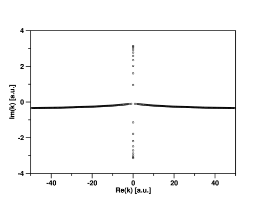
Figure 1: The complex $k$ spectrum for a particle in the step potential of Eq. (1) with $V_{0}=5$ and $a=10$. The spectrum is entirely discrete. Ten bound states [$\mathrm{Re}(k)=0$, $\mathrm{Im}(k)>0$] are present, as well as nine antibound [$\mathrm{Re}(k)=0$, $\mathrm{Im}(k)<0$]. The positive $\mathrm{Re}(k)$ branch of the spectrum shows the complex wave numbers of the outgoing Siegert pseudostates, the negative $\mathrm{Re}(k)$ branch the incoming.

This transcendental equation can be solved for only a discrete set of $k$ values. As was done, for instance, in Ref. KoMo84 , we solve Eq. (3) numerically, after setting $V_{0}=5$ and $a=10$. The resulting discrete $k$ spectrum is presented in Fig. 1. There are $10$ bound states, which appear on the positive imaginary axis. The nine antibound states lie on the negative imaginary axis. The solutions with $\mathrm{Re}(k)>0$ are associated with outgoing Siegert pseudostates. Similarly, states with $\mathrm{Re}(k)<0$ refer to incoming Siegert pseudostates.

Traditionally, Siegert-state theory has focused on scattering resonances and decaying states. See Refs. Newt02 ; MoGe73 ; ToOs97 ; ToOs98 for an overview of the literature. Several methods exist that allow one to directly calculate the complex energy of a decaying state: complex scaling Rein82 ; Mois98 ; ReMc78 , complex absorbing potentials SaCe02 ; RiMe93 , and the direct solution of the Schrödinger equation subject to the Siegert boundary condition, Eq. (2). This third approach used to be numerically inefficient, because a nonlinear eigenvalue problem had to be solved in an iterative fashion BaJu72 ; McRe79 ; Schn81 .

A major step forward was made by Tolstikhin, Ostrovsky, and Nakamura ToOs97 ; ToOs98 . Their method provides, after solving a single generalized eigenvalue problem, access not only to the bound, antibound, and resonance states, but also to the discretized pseudocontinuum. In addition, it becomes possible to derive fundamental properties of Siegert pseudostates using simple and elegant mathematical techniques. An application of the method of Refs. ToOs97 ; ToOs98 to a molecular fragmentation problem is the subject of Ref. HaGr02 . In that work, only bound states and outgoing Siegert pseudostates were utilized as fragmentation-channel basis functions.

A point of central concern in this paper is the time evolution of a wave packet expanded in terms of Siegert pseudostates. This aspect was first addressed by Yoshida et al. YoWa99 . They successfully introduced Siegert pseudostates as a basis capable of eliminating artificial boundary reflections. In a subsequent paper TaWa01 , it is argued that the time evolution for $t>0$ is given by

$$\psi(r;t)=\sum_{n}(\varphi_{n}|\psi)\mathrm{e}^{-\mathrm{i}E_{n}t}\varphi_{n}(r)\;,$$ (4)

where the imaginary part of the complex energy $E_{n}$ is negative. $\varphi_{n}(r)$ is the spatial representation of the $n$th Siegert pseudostate, and

$$(\varphi_{n}|\psi)=\int_{0}^{a}\varphi_{n}(r)\psi(r;t=0)\mathrm{d}r\;.$$ (5)

In Sec. II, we review some ideas of the formalism of Tolstikhin, Ostrovsky, and Nakamura. We extend their work by providing arguments why certain subsets of Siegert pseudostates may be employed as bases. Moreover, we investigate time evolution in the context of Siegert pseudostates. We find that rigorous Siegert-pseudostate theory, in general, necessitates nonexponential time evolution, in contradiction to Eq. (4). Numerical evidence is presented in Sec. III. The calculations demonstrate that for a fast-moving wave packet Eq. (4) is accurate, while its performance deteriorates as the average energy of the wave packet is decreased. Section IV concludes. Atomic units are used throughout.

II Mathematical considerations

Consider the radial Schrödinger equation

$$\hat{H}\varphi(r)=E\varphi(r)\;,$$ (6)

where

$$\hat{H}=-\frac{1}{2}\frac{\mathrm{d}^{2}}{\mathrm{d}r^{2}}+V(r)\;.$$ (7)

$V(r)$ is an arbitrary (short-range) potential. We seek solutions $\varphi(r)$ for $r\in[0,a]$ ($a>0$), such that at $r=0$ the usual boundary condition for the radial eigenvalue problem

$$\varphi(0)=0$$ (8)

and at $r=a$ the Siegert boundary condition, Eq. (2), are satisfied. The solutions $\varphi(r)$ are referred to as Siegert pseudostates ToOs97 ; ToOs98 . Equation (2) allows us to separate solutions to the Schrödinger equation into purely outgoing, purely incoming, bound, and antibound states.

The wave number $k$ in Eq. (2) is in general complex. Its relation to the eigenenergy $E$ is given by

$$E=\frac{k^{2}}{2}+V(a)\;,$$ (9)

which implies that $a$ should be chosen sufficiently large, if possible, such that $V(r)=\mathrm{const.}$ for $r\geq a$. Applying Eq. (9) in the case of a long-range potential introduces the approximation of forcing the potential to be constant beyond $r=a$, while preserving continuity of the potential at that point—in contrast to the approach taken in Ref. ToOs97 ; ToOs98 , which enforces a discontinuity by setting $V(a)=0$ in Eq. (9).

Utilizing a set of $N$ linearly independent, not necessarily orthogonal basis functions $\{y_{j}(r):j=1,\ldots,N\}$ on the interval $[0,a]$ and assuming completeness in the limit $N\rightarrow\infty$, we can make the ansatz

$$\varphi(r)=\sum_{j=1}^{N}c_{j}y_{j}(r)\;.$$ (10)

If we insert this into Eq. (6), multiply from the left by $y_{i}(r)$, and integrate over $r$ from $0$ to $a$, we find

$$-\frac{1}{2}\int_{0}^{a}y_{i}(r)\frac{\mathrm{d}^{2}}{\mathrm{d}r^{2}}\sum_{j=1}^{N}c_{j}y_{j}(r)\mathrm{d}r+\int_{0}^{a}y_{i}(r)V(r)\sum_{j=1}^{N}c_{j}y_{j}(r)\mathrm{d}r=E\int_{0}^{a}y_{i}(r)\sum_{j=1}^{N}c_{j}y_{j}(r)\mathrm{d}r$$ (11)

The term containing the second derivative with respect to $r$ can be integrated by parts. Thus, after applying the boundary conditions in Eqs. (8) and (2), we define

$$\tilde{H}_{ij} = \int_{0}^{a}\frac{\mathrm{d}}{\mathrm{d}r}y_{i}(r)\frac{\mathrm{d}}{\mathrm{d}r}y_{j}(r)\mathrm{d}r$$

$$+2\int_{0}^{a}y_{i}(r)[V(r)-V(a)]y_{j}(r)\mathrm{d}r\;,$$

$$S_{ij} = \int_{0}^{a}y_{i}(r)y_{j}(r)\mathrm{d}r\;,$$ (13)

$$L_{ij} = y_{i}(a)y_{j}(a)\;,$$ (14)

$$\varkappa = \mathrm{i}k\;,$$ (15)

and arrive at the nonlinear eigenvalue problem

$$\left(\tilde{\bm{H}}+\varkappa^{2}{\bm{S}}-\varkappa{\bm{L}}\right){\bm{c}}={\bm{0}}\;.$$ (16)

We refer to the eigenvector ${\bm{c}}$ in this equation as Siegert pseudovector. In practical calculations, the basis functions $y_{j}(r)$ may be chosen to be real. Thus, the matrices $\tilde{\bm{H}}$, ${\bm{S}}$, and ${\bm{L}}$ may be assumed to be symmetric and elements of $\mathbb{R}^{N\times N}$. Note, however, that the vector ${\bm{c}}$, consisting of the expansion coefficients $c_{j}$, $j=1,\ldots,N$ [see Eq. (10)], is complex in general: ${\bm{c}}\in\mathbb{C}^{N}$. If Eq. (16) is satisfied by an eigenpair $(\varkappa,{\bm{c}})$, then—in view of the realness of $\tilde{\bm{H}}$, ${\bm{S}}$, and ${\bm{L}}$—the pair $(\varkappa^{\ast},{\bm{c}}^{\ast})$ also forms a solution.

Tolstikhin, Ostrovsky, and Nakamura ToOs97 ; ToOs98 observed that the nonlinear eigenvalue problem of Eq. (16) can be recast in terms of a linear one by defining

$${\bm{d}}=\varkappa{\bm{c}}\;.$$ (17)

Then, Eq. (16) goes over into

$$-\tilde{\bm{H}}{\bm{c}}=\varkappa\left({\bm{S}}{\bm{d}}-{\bm{L}}{\bm{c}}\right)\;,$$ (18)

and, trivially,

$${\bm{S}}{\bm{d}}=\varkappa{\bm{S}}{\bm{c}}\;.$$ (19)

These two matrix equations are equivalent to the generalized eigenvalue problem

$${\bm{A}}{\bm{x}}=\varkappa{\bm{B}}{\bm{x}}\;.$$ (20)

The symmetric matrices ${\bm{A}}$ and ${\bm{B}}$ $\in\mathbb{R}^{2N\times 2N}$ are given by

$${\bm{A}}=\left[\begin{array}[]{cc}-\tilde{\bm{H}}&{\bm{0}}\\ {\bm{0}}&{\bm{S}}\end{array}\right]\;,$$ (21)

$${\bm{B}}=\left[\begin{array}[]{cc}-{\bm{L}}&{\bm{S}}\\ {\bm{S}}&{\bm{0}}\end{array}\right]\;,$$ (22)

and the eigenvector ${\bm{x}}\in\mathbb{C}^{2N}$ in Eq. (20) is composed of the two vectors ${\bm{c}}$ and ${\bm{d}}$:

$${\bm{x}}=\left[\begin{array}[]{c}{\bm{c}}\\ {\bm{d}}\end{array}\right]\;.$$ (23)

Let us denote by $\tilde{N}$ the number of linearly independent solutions ${\bm{x}}_{n}$ (eigenvalue $\varkappa_{n}$) to the generalized eigenvalue problem in Eq. (20). (It is by no means clear that $\tilde{N}=2N$.) We then define the matrices

$${\bm{X}}=[{\bm{x}}_{1},\ldots,{\bm{x}}_{\tilde{N}}]\in\mathbb{C}^{2N\times\tilde{N}}$$ (24)

and

$${\bm{K}}=\mathrm{diag}(\varkappa_{1},\ldots,\varkappa_{\tilde{N}})\in\mathbb{C}^{\tilde{N}\times\tilde{N}}\;,$$ (25)

such that

$${\bm{A}}{\bm{X}}={\bm{B}}{\bm{X}}{\bm{K}}\;.$$ (26)

The overlap matrix ${\bm{S}}$ [Eq. (13)] is positive-definite and therefore invertible. Its inverse, ${\bm{S}}^{-1}$, is also symmetric. It can be concluded that the inverse of ${\bm{B}}$ exists, since it is easily seen by direct construction that

$${\bm{B}}^{-1}=\left[\begin{array}[]{cc}{\bm{0}}&{\bm{S}}^{-1}\\ {\bm{S}}^{-1}&{\bm{S}}^{-1}{\bm{L}}{\bm{S}}^{-1}\end{array}\right]\;.$$ (27)

The real symmetric matrix ${\bm{B}}$ can be diagonalized via an orthogonal similarity transformation,

$${\bm{U}}^{\mathrm{T}}{\bm{B}}{\bm{U}}={\bm{D}}\;,$$ (28)

where ${\bm{U}}\in\mathbb{R}^{2N\times 2N}$ is orthogonal, ${\bm{U}}^{\mathrm{T}}{\bm{U}}={\bm{\openone}}$, and ${\bm{D}}\in\mathbb{R}^{2N\times 2N}$ is diagonal. All diagonal elements of ${\bm{D}}$ differ from zero, for ${\bm{D}}$ is similar to ${\bm{B}}$ and thus also invertible. With this in mind, the matrix

$$\tilde{\bm{U}}={\bm{U}}{\bm{D}}^{-1/2}\in\mathbb{C}^{2N\times 2N}$$ (29)

can be introduced in a meaningful way. While ${\bm{B}}$ is invertible [Eq. (27)], it is in general neither positive- nor negative-definite. Hence, some of the columns of $\tilde{\bm{U}}$ are real, but the others are purely imaginary. The matrix $\tilde{\bm{U}}$ can be utilized to convert the real symmetric, indefinite generalized eigenvalue problem, Eq. (26), to a standard one:

$$\tilde{\bm{A}}\tilde{\bm{X}}=\tilde{\bm{X}}{\bm{K}}\;.$$ (30)

Here,

$$\tilde{\bm{A}}=\tilde{\bm{U}}^{\mathrm{T}}{\bm{A}}\tilde{\bm{U}}$$ (31)

and

$$\tilde{\bm{X}}={\bm{D}}\tilde{\bm{U}}^{\mathrm{T}}{\bm{X}}\;.$$ (32)

The matrix $\tilde{\bm{A}}$ is complex symmetric. Unfortunately, complex symmetry is not a very useful property, as it is known that any complex matrix of square format is similar to a complex symmetric matrix (see, for instance, Ref. SaCe02 ). Generally, it is not possible to guarantee diagonalizability, i.e. the existence of a basis of eigenvectors, of a complex symmetric matrix. Note that $\tilde{\bm{A}}$ consists of purely real and purely imaginary matrix blocks, but whether this helps to prove its diagonalizability is currently unclear. A sufficient condition for diagonalizability is that all $2N$ eigenvalues $\varkappa_{n}$ are distinct. Degeneracies could cause difficulties, but in numerical calculations true (accidental) degeneracies are practically never encountered. Under the assumption that $\tilde{\bm{A}}$ is diagonalizable, $\tilde{N}=2N$ and the matrix

$$\tilde{\bm{X}}=[\tilde{\bm{x}}_{1},\ldots,\tilde{\bm{x}}_{2N}]\in\mathbb{C}^{2N\times 2N}$$ (33)

may be chosen to be complex orthogonal,

$$\tilde{\bm{X}}^{\mathrm{T}}\tilde{\bm{X}}={\bm{\openone}}\;,$$ (34)

as shown, e.g., in Ref. SaCe02 . The $2N$ vectors $\tilde{\bm{x}}_{n}$ are linearly independent and, consequently, form a basis of $\mathbb{C}^{2N}$. This fact can be expressed in compact form in terms of the completeness relation

$$\sum_{n=1}^{2N}\tilde{\bm{x}}_{n}\tilde{\bm{x}}_{n}^{\mathrm{T}}={\bm{\openone}}\;.$$ (35)

From Eqs. (34) and (35) it follows for the solutions ${\bm{x}}_{n}$ of the original generalized eigenvalue problem in Eq. (20) that

$${\bm{x}}_{m}^{\mathrm{T}}{\bm{B}}{\bm{x}}_{n}=\delta_{mn}\;,\;m,n=1,\ldots,2N\;,$$ (36)

and

$$\sum_{n=1}^{2N}{\bm{x}}_{n}{\bm{x}}_{n}^{\mathrm{T}}={\bm{B}}^{-1}\;.$$ (37)

Combining Eq. (36) with Eqs. (17), (22), and (23), and employing the normalization convention of Refs. ToOs97 ; ToOs98 , the orthonormality relation satisfied by the eigenvectors ${\bm{c}}_{n}$ of the nonlinear eigenvalue problem in Eq. (16) reads

$${\bm{c}}_{m}^{\mathrm{T}}{\bm{S}}{\bm{c}}_{n}-\frac{{\bm{c}}_{m}^{\mathrm{T}}{\bm{L}}{\bm{c}}_{n}}{\varkappa_{m}+\varkappa_{n}}=\delta_{mn}\;,\;m,n=1,\ldots,2N\;.$$ (38)

Take notice of the occurrence of a singularity in this expression if $\varkappa_{m}+\varkappa_{n}$ approaches $0$ for some pair of indices $m,n$. This happens whenever there is a deeply bound state (eigenvalue $\varkappa_{m}$), since there exists a corresponding antibound state whose eigenvalue $\varkappa_{n}$ equals $-\varkappa_{m}$ to machine precision.

Even in the absence of the term involving the surface matrix ${\bm{L}}$, Eq. (38) could not be used to establish a proper inner product on $\mathbb{C}^{N}$, because, for a given vector ${\bm{v}}\in\mathbb{C}^{N}\setminus\{{\bm{0}}\}$, ${\bm{v}}^{\mathrm{T}}{\bm{S}}{\bm{v}}$ is not necessarily different from zero. The occurrence of indefinite inner products is also well known in the context of complex scaling Rein82 ; Mois98 and in the method of complex absorbing potentials SaCe02 ; RiMe93 . The following three relations are consequences of Eqs. (17), (23), (27), and (37):

$$\sum_{n=1}^{2N}\frac{1}{\varkappa_{n}}{\bm{c}}_{n}{\bm{c}}_{n}^{\mathrm{T}} = {\bm{0}}\;,$$ (39)

$$\sum_{n=1}^{2N}{\bm{c}}_{n}{\bm{c}}_{n}^{\mathrm{T}} = 2{\bm{S}}^{-1}\;,$$ (40)

$$\sum_{n=1}^{2N}\varkappa_{n}{\bm{c}}_{n}{\bm{c}}_{n}^{\mathrm{T}} = 2{\bm{S}}^{-1}{\bm{L}}{\bm{S}}^{-1}\;.$$ (41)

The normalization suggested by Eq. (38) has been applied.

Equation (40) demonstrates that any vector ${\bm{v}}\in\mathbb{C}^{N}$ can be represented as a superposition of the Siegert pseudovectors ${\bm{c}}_{n}$:

$${\bm{v}}=\frac{1}{2}\sum_{n=1}^{2N}\left({\bm{c}}_{n}^{\mathrm{T}}{\bm{S}}{\bm{v}}\right){\bm{c}}_{n}\;.$$ (42)

This representation, however, is not unique, for the vectors ${\bm{c}}_{n}$, $n=1,\ldots,2N$, form an overcomplete subset of $\mathbb{C}^{N}$. The rank of the matrix ${\bm{C}}=[{\bm{c}}_{1},\ldots,{\bm{c}}_{2N}]\in\mathbb{C}^{N\times 2N}$ cannot be greater than $N$ [in fact, because of Eq. (40), $\mathrm{rank}({\bm{C}})=N$]. Thus, the vectors ${\bm{c}}_{1},\ldots,{\bm{c}}_{2N}$ are linearly dependent, i.e., the equation

$$\sum_{n=1}^{2N}\alpha_{n}{\bm{c}}_{n}={\bm{0}}$$ (43)

can be satisfied by some $\alpha_{n}\neq 0$. If we define

$$M_{mn}={\bm{c}}_{m}^{\mathrm{T}}{\bm{S}}{\bm{c}}_{n}\;,$$ (44)

then

$$\sum_{n=1}^{2N}M_{mn}\alpha_{n}=0\;,m=1,\ldots,2N\;,$$ (45)

from which we may conclude that the matrix ${\bm{M}}\in\mathbb{C}^{2N\times 2N}$ cannot be invertible (since not all $\alpha_{n}$ have to be equal to $0$). The nonuniqueness of the representation in Eq. (42) is directly linked to the noninvertibility of ${\bm{M}}$.

Another instructive way of looking at this is to make use of Eq. (40) to derive the following relation:

$${\bm{M}}{\bm{M}}=2{\bm{M}}\;.$$ (46)

If ${\bm{M}}$ were invertible, then we would have ${\bm{M}}=2{\bm{\openone}}$. This contradicts the orthonormality relation, Eq. (38):

$$M_{mn}=\delta_{mn}+\frac{{\bm{c}}_{m}^{\mathrm{T}}{\bm{L}}{\bm{c}}_{n}}{\varkappa_{m}+\varkappa_{n}}\;.$$ (47)

For example, for $m=n$ the surface term can be written as $\varphi_{m}(a)^{2}/2\varkappa_{m}$ [Eqs. (10) and (14)], which differs from unity in general.

In Appendix A, we demonstrate that a subset of $\{{\bm{c}}_{1},\ldots,{\bm{c}}_{2N}\}$ can be found, comprising exactly $N$ vectors and forming a basis of $\mathbb{C}^{N}$. Without loss of generality, the elements of this subset are taken to be the vectors ${\bm{c}}_{1},\ldots,{\bm{c}}_{N}$. The proper completeness relation allows one to represent an arbitrary vector ${\bm{v}}\in\mathbb{C}^{N}$ in a unique way:

$${\bm{v}}=\sum_{n=1}^{N}\alpha_{n}{\bm{c}}_{n}\;.$$ (48)

Necessarily,

$$\sum_{n=1}^{N}M_{mn}\alpha_{n}={\bm{c}}_{m}^{\mathrm{T}}{\bm{S}}{\bm{v}}\;,m=1,\ldots,N\;.$$ (49)

Note that the matrix elements $M_{mn}$ in this equation refer only to the selected subset. The linear independence of the Siegert pseudovectors ${\bm{c}}_{1},\ldots,{\bm{c}}_{N}$ ensures the invertibility of ${\bm{M}}\in\mathbb{C}^{N\times N}$ [cf. Eqs. (43), (44), and (45)]. The expansion coefficients $\alpha_{m}$ are unique and are given by

$$\alpha_{m}=\sum_{n=1}^{N}\left({\bm{M}}^{-1}\right)_{mn}{\bm{c}}_{n}^{\mathrm{T}}{\bm{S}}{\bm{v}}\;.$$ (50)

The associated completeness relation reads

$$\sum_{m=1}^{N}\sum_{n=1}^{N}{\bm{c}}_{m}\left({\bm{M}}^{-1}\right)_{mn}{\bm{c}}_{n}^{\mathrm{T}}={\bm{S}}^{-1}\;.$$ (51)

Let us now turn our attention to the problem of describing the time evolution of an outgoing wave packet utilizing Siegert pseudostates. For that purpose, it is natural to choose for the basis $\{{\bm{c}}_{1},\ldots,{\bm{c}}_{N}\}$ all outgoing Siegert pseudovectors [$\mathrm{Re}(k_{n})>0$] plus a complementary number of bound eigenvectors. (We provide in Sec. III numerical evidence that these form indeed a basis of $\mathbb{C}^{N}$.) Consider an initial wave packet $\psi(r;t=0)$ that is entirely localized within the interval $[0,a]$. Using Eqs. (10) and (51), and assuming pure exponential time evolution for each Siegert pseudostate, the time evolution of the wave packet for $t>0$ is obtained from

$$\psi(r;t)=\sum_{m=1}^{N}\sum_{n=1}^{N}\left({\bm{M}}^{-1}\right)_{mn}(\varphi_{n}|\psi)\mathrm{e}^{-\mathrm{i}E_{m}t}\varphi_{m}(r)\;,$$ (52)

where

$$E_{m}=\frac{k_{m}^{2}}{2}+V(a)\;.$$ (53)

One disadvantage of Eq. (52) is the need to invert a matrix. In addition, as we will see below, the assumption of exponential time evolution is wrong in general for Siegert pseudostates.

A practically and formally more acceptable expression for the time evolution of the wave packet can be derived from the Mittag-Leffler partial fraction decomposition NaNi01 of the outgoing-wave Green’s function represented with respect to Siegert pseudostates. This representation has been given in Refs. MoGe73 ; ToOs97 ; ToOs98 . The outgoing-wave Green’s function satisfies the equations

$$(E-\hat{H})G(r,r^{\prime};k) = \delta(r-r^{\prime})\;,$$ (54)

$$G(0,r^{\prime};k) = 0\;,$$ (55)

$$\left.\frac{\mathrm{d}}{\mathrm{d}r}G(r,r^{\prime};k)\right|_{r=a} = \mathrm{i}kG(a,r^{\prime};k)\;,$$ (56)

for $r,r^{\prime}\in[0,a]$. These conditions can be translated to

$$\left(\tilde{\bm{H}}+\varkappa^{2}{\bm{S}}-\varkappa{\bm{L}}\right){\bm{G}}(k)=-2{\bm{\openone}}\;,$$ (57)

where the matrix representation of the outgoing-wave Green’s function in the basis of the functions $y_{j}(r)$ is defined via the relation

$$G(r,r^{\prime};k)=\sum_{i=1}^{N}\sum_{j=1}^{N}G_{ij}(k)y_{i}(r)y_{j}(r^{\prime})\;.$$ (58)

Making the ansatz

$${\bm{G}}(k)=\sum_{n=1}^{2N}\alpha_{n}{\bm{c}}_{n}{\bm{c}}_{n}^{\mathrm{T}}$$ (59)

and putting Eqs. (39), (40) to use, it follows from Eq. (57) that

$$\alpha_{n}=\frac{1}{k_{n}(k-k_{n})}\;.$$ (60)

Hence,

$$G(r,r^{\prime};k)=\sum_{n=1}^{2N}\frac{\varphi_{n}(r)\varphi_{n}(r^{\prime})}{k_{n}(k-k_{n})}\;,\;r,r^{\prime}\in[0,a]\;,$$ (61)

serves as an approximation to the outgoing-wave Green’s function, within the framework of the underlying finite basis set $\{y_{j}(r):j=1,\ldots,N\}$.

The Green’s function in Eq. (61) allows us to determine the time evolution of the wave packet for $t>0$ GoWa64 :

$$\psi(r;t)=\frac{\mathrm{i}}{2\pi}\int_{-\infty}^{\infty}\mathrm{d}E\,\mathrm{e}^{-\mathrm{i}Et}\int_{0}^{a}\mathrm{d}r^{\prime}G(r,r^{\prime};k)\psi(r^{\prime};t=0)=\sum_{n=1}^{2N}\beta_{n}(t)(\varphi_{n}|\psi)\varphi_{n}(r)\;.$$ (62)

Here,

$$\beta_{n}(t)=\frac{\mathrm{i}}{2\pi}\int_{-\infty}^{\infty}\frac{\mathrm{e}^{-\mathrm{i}Et}}{k_{n}(k-k_{n})}\mathrm{d}E\;.$$ (63)

The integration path lies on the physical sheet Newt02 of the energy Riemann surface, and runs from $-\infty$ to $+\infty$ infinitesimally above the real $E$ axis GoWa64 . In order to evaluate $\beta_{n}(t)$, we use Eq. (9) and replace the integration path in the energy plane by the integration contour in the complex $k$ plane illustrated in Fig. 2a. For $t<0$, this contour can be closed in the first quadrant of the $k$ plane without affecting $\beta_{n}(t)$. The resulting integration loop is indicated in Fig. 2b. The integration path along the positive imaginary axis is infinitesimally displaced toward positive real $k$ values, so that the integrand in Eq. (63) is analytic on and inside the loop. Hence, $\beta_{n}(t)=0$ for $t<0$, as expected for a description based on the outgoing-wave Green’s function.

Figure 2: a) The integration contour in the complex $k$ plane employed to evaluate Eq. (63). The integration proceeds along the imaginary axis from $\mathrm{i}\infty$ to the origin, and from there along the real axis to $+\infty$. This contour corresponds to integration from $-\infty$ to $+\infty$ on the physical sheet of the energy Riemann surface. b) If $t<0$, then the contour may be closed in the first quadrant of the $k$ plane. c) The integration path in a) may be evaluated for $t>0$ using one closed contour and one that runs from $-\infty$ to $+\infty$.

If $t>0$, then $\beta_{n}(t)$ can be written as the sum of two separate contour integrals. The respective contours are shown in Fig. 2c. Thus we have

$$\beta_{n}(t)=\beta_{n}^{(I)}(t)+\beta_{n}^{(II)}(t)\;,$$ (64)

where

$$\beta_{n}^{(I)}(t)=\left\{\begin{array}[]{ll}\mathrm{e}^{-\mathrm{i}E_{n}t}&\textrm{for bound states}\\ 0&\textrm{otherwise}\end{array}\right.$$ (65)

and

$$\beta_{n}^{(II)}(t) = \frac{\mathrm{i}}{2\pi}\frac{\exp{\left\{-\mathrm{i}V(a)t\right\}}}{k_{n}}\int_{-\infty}^{\infty}\frac{k}{k-k_{n}}\mathrm{e}^{-\mathrm{i}k^{2}t/2}\mathrm{d}k$$

$$= \frac{\mathrm{i}}{2\pi}\exp{\left\{-\mathrm{i}V(a)t\right\}}$$

$$\times\left\{\frac{\mathrm{e}^{-\mathrm{i}\pi/4}}{k_{n}}\sqrt{\frac{2\pi}{t}}+\int_{-\infty}^{\infty}\frac{\mathrm{e}^{-\mathrm{i}k^{2}t/2}}{k-k_{n}}\mathrm{d}k\right\}\;.$$

From Eq. (39) it follows that

$$\sum_{n=1}^{2N}\frac{1}{k_{n}}(\varphi_{n}|\psi)\varphi_{n}(r)=0\;.$$ (67)

Therefore, the term proportional to $t^{-1/2}$ in $\beta_{n}^{(II)}(t)$ does not contribute to $\psi(r;t)$, Eq. (62), and we will not consider it further. As demonstrated in Appendix B, the integral in Eq. (II) can be expressed utilizing the Faddeeva function FaTe61 ; FrCo61 ; Huml79 ; NeAg81 ; PoWi90 ; SuTh91 ; Well99

$$w(z)=\frac{\mathrm{i}}{\pi}\int_{-\infty}^{\infty}\frac{\mathrm{e}^{-s^{2}}}{z-s}\mathrm{d}s\;,\;\mathrm{Im}(z)>0\;.$$ (68)

Hence, on combining Eqs. (64), (65), (II), and the results from Appendix B, the time-evolution coefficients $\beta_{n}(t)$, $t>0$, read

$$\beta_{n}(t)=\exp{\left\{-\mathrm{i}V(a)t\right\}}\times\left\{\begin{array}[]{ll}\mathrm{e}^{-\mathrm{i}k_{n}^{2}t/2}-\frac{1}{2}w\left(\mathrm{e}^{\mathrm{i}\pi/4}\sqrt{\frac{t}{2}}k_{n}\right)&\;\textrm{for bound or outgoing states}\\ \\ \frac{1}{2}w\left(-\mathrm{e}^{\mathrm{i}\pi/4}\sqrt{\frac{t}{2}}k_{n}\right)&\;\textrm{for antibound or incoming states}\end{array}\right.\;.$$ (69)

(The square root in the argument of the Faddeeva function must be interpreted as a positive number.) The result in Eq. (69), together with Eq. (62), represents—within the framework of Siegert pseudostates—the most consistent approach to describing the time evolution of a wave packet. It is interesting to observe that in the limit $t\rightarrow 0^{+}$, all $\beta_{n}(t)$ tend to $1/2$, for the Faddeeva function goes to unity in this limit. This ensures, in view of Eq. (40), that $\lim_{t\rightarrow 0^{+}}\psi(r;t)=\psi(r;t=0)$. Equations (62) and (69) also allow us to determine the long-term behavior of the wave packet in the interval $[0,a]$. Using the asymptotic expansion of the Faddeeva function AbSt70 and Eq. (67), the wave packet for large $t$ is seen to consist of bound-state components evolving according to the $\exp{\left\{-\mathrm{i}E_{n}t\right\}}$ factor in Eq. (69) as well as a decaying component that evolves in time as $t^{-3/2}$. This specific power-law behavior of a decaying state—in the long-time limit—is in fact well known MoGe73 ; GoWa64 ; JaSa61 ; Wint61 ; DiRe02 (see Refs. NiBe77 ; Nico02 for an alternative view).

III Numerical Studies

In this section, we apply the techniques developed so far to a wave packet in the model potential of Eq. (1) [$V_{0}=5$ and $a=10$]. For the basis $\{y_{j}(r):j=1,\ldots,N\}$, a finite-element basis set based on fifth-order Hermite interpolating polynomials was used Bath76 ; BaWi76 ; BrSc93 ; AcSh96 ; ReBa97 ; MeGr97 ; SaCh04 . A mesh of evenly-spaced nodes was defined radially, with three finite elements centered at the $i$th node, $r_{i}$. All three vanish in $[0,r_{i-1}]$ and $[r_{i+1},a]$. Their behavior at $r_{i}$ separates them into three types. The zero-type polynomials have a finite function value at the $i$th node, but zero first and second derivatives. The one-type have a finite first derivative, but zero function value and zero second derivative. The two-type have a finite curvature, but vanishing zero and first derivatives. In order to enforce vanishing at the origin, Eq. (8), only the one- and two-types are considered at the first node (at $r=0$). Thus, the dimension of the finite-element basis set ($N$) is equal to one less than three times the number of nodes.

We numerically Lapa99 solve the generalized eigenvalue problem of Eq. (20) to obtain $2N$ Siegert pseudostates with $2N$ distinct eigenvalues $\varkappa_{n}$. Appendix A proves that certain subsets of $N$ Siegert pseudostates achieve completeness in $\mathbb{C}^{N}$. However, which $N$ states must be selected is not clear. By looking at the eigenvalues of the matrix ${\bm{M}}\in\mathbb{C}^{N\times N}$ [Eq. (44)], one can determine whether or not a selected subset of $N$ vectors is complete. If the vectors form a basis, the ${\bm{M}}$ matrix will have $N$ (not necessarily distinct) eigenvalues which differ from zero. For the potential under consideration, the number of bound states equals the number of antibound states. (In the Introduction, we mentioned that there are $10$ physical bound and nine physical antibound states. The $10$th antibound state found in the numerical calculation cannot be converged and does not correspond to an eigenstate of the Hamiltonian.) All combinations of bound or antibound with incoming or outgoing Siegert pseudostates supply $N$ distinct vectors, giving four plausible choices for a complete, useful basis set. The eigenvalues of ${\bm{M}}$ were calculated for each case, and in so far as zero was never one of them, all combinations proved to span $\mathbb{C}^{N}$. More specifically, more than $95$ % of all eigenvalues of ${\bm{M}}$ equal unity to machine precision. The rest have a magnitude ranging from $0.93$ to $230$.

To assess the ability of the Siegert pseudostates to represent a wave packet at $t=0$, it is first necessary to investigate the limiting accuracy of the underlying finite-element basis set. An initial wave packet is given the form of a Gaussian multiplied by a plane wave:

$$\psi(r;t=0)=\exp{[-\frac{\left(r-r_{0}\right)^{2}}{2\xi^{2}}+\mathrm{i}k_{0}\left(r-r_{0}\right)]}\;.$$ (70)

The Gaussian is centered in the middle of the well at $r_{0}=5$, and $\xi=0.5$ is chosen to ensure that contribution outside the interval $[0,a]$ is negligible.

We represent the wave packet as a superposition of the finite elements,

$$\psi(r;t=0)\approx\sum_{j=1}^{N}\alpha_{j}y_{j}(r)\;,$$ (71)

where the expansion coefficients are chosen to minimize

$$\chi_{1}^{2}=\int_{0}^{a}\left|\psi(r;t=0)-\sum_{j=1}^{N}\alpha_{j}y_{j}(r)\right|^{2}\mathrm{d}r\;,$$ (72)

i.e.,

$$\alpha_{i}=\sum_{j=1}^{N}\left({\bm{S}}^{-1}\right)_{ij}\int_{0}^{a}y_{j}(r)\psi(r;t=0)\mathrm{d}r\;.$$ (73)

On the basis of $\chi_{1}^{2}$, we determine how accurately our finite set of piecewise-defined polynomials is able to approximate a specific element of the infinite-dimensional Hilbert space.

Let us next consider the completeness relation expressed by Eq. (51). The set of $N$ selected Siegert pseudostates must be capable of representing the unique coefficient vector ${\bm{\alpha}}\in\mathbb{C}^{N}$,

$$\tilde{\bm{\alpha}}=\sum_{n=1}^{N}\gamma_{n}{\bm{c}}_{n}\;,$$ (74)

where, ideally, $\tilde{\bm{\alpha}}={\bm{\alpha}}$. According to Eq. (51),

$$\gamma_{m}=\sum_{n=1}^{N}\left({\bm{M}}^{-1}\right)_{mn}{\bm{c}}_{n}^{\mathrm{T}}{\bm{S}}{\bm{\alpha}}\;.$$ (75)

The quality of the Siegert pseudovector expansion is measured by

$$\chi_{2}^{2}=\sum_{j=1}^{N}|\alpha_{j}-\tilde{\alpha}_{j}|^{2}\;.$$ (76)

Now with the expansion coefficients themselves superpositions of the Siegert pseudostates, we calculate

$$\chi_{3}^{2}=\int_{0}^{a}\left|\psi(r;t=0)-\sum_{n=1}^{N}\gamma_{n}\varphi_{n}(r)\right|^{2}\mathrm{d}r$$ (77)

to test the ability of the chosen subset of $N$ Siegert pseudostates to accurately reproduce the wave packet at $t=0$.

We now focus on Eq. (40), which allows us to expand the wave packet in terms of all $2N$ Siegert pseudostates:

$$\chi_{4}^{2}=\sum_{j=1}^{N}\left|\alpha_{j}-\sum_{n=1}^{2N}\zeta_{n}c_{jn}\right|^{2}\;,$$ (78)

$$\zeta_{n}=\frac{1}{2}{\bm{c}}_{n}^{\mathrm{T}}{\bm{S}}{\bm{\alpha}}\;,$$ (79)

$$\chi_{5}^{2}=\int_{0}^{a}\left|\psi(r;t=0)-\sum_{n=1}^{2N}\zeta_{n}\varphi_{n}(r)\right|^{2}\mathrm{d}r\;.$$ (80)

Table 1: The $\chi^{2}$’s described in Eqs. (72)-(80), as a function of finite-element basis size, $N$, calculated for the case where $k_{0}=15$ in Eq. (70). $\chi_{1}^{2}$ demonstrates convergence to accurate wave-packet reproduction as the number of finite-element basis functions is increased. $\chi_{2}^{2}$ and $\chi_{4}^{2}$ show the ability of the expansions of Eqs. (52) and (62), respectively, to match the unique coefficients of Eq. (73). $\chi_{3}^{2}$ and $\chi_{5}^{2}$ confirm that these expansions are successful in reproducing the initial wave packet at the level limited by the underlying finite elements. Notation $x[y]$ stands for $x\times 10^{y}$.

$N$	$\chi_{1}^{2}$	$\chi_{2}^{2}$	$\chi_{3}^{2}$	$\chi_{4}^{2}$	$\chi_{5}^{2}$
$20$	$0.89$	$2.7[-19]$	$0.89$	$9.6[-20]$	$0.89$
$80$	$1.5[-3]$	$1.4[-17]$	$1.5[-3]$	$2.2[-19]$	$1.5[-3]$
$200$	$2.0[-7]$	$4.5[-20]$	$2.0[-7]$	$5.3[-21]$	$2.0[-7]$
$380$	$3.0[-11]$	$7.8[-20]$	$3.0[-11]$	$9.8[-21]$	$3.0[-11]$
$620$	$5.5[-14]$	$4.5[-18]$	$5.5[-14]$	$9.9[-19]$	$5.5[-14]$

All five $\chi^{2}$’s were calculated as a function of $N$, the number of finite-element basis functions, with $k_{0}=15$ [see Eq. (70)]. The values are displayed in Table 1. Only $\chi_{2}^{2}$’s and $\chi_{3}^{2}$’s using bound and outgoing Siegert pseudostates are tabulated, since these states provided the qualitatively best results for time evolution based on Eq. (52). Other combinations of $N$ Siegert pseudostates will not be discussed further.

One observes in Table 1 that as the number of basis functions being used is increased, $\chi_{1}^{2}$ approaches convergence. For all values of $N$, the high accuracy of $\chi_{2}^{2}$ confirms that the Siegert pseudovectors indeed form a basis for $\mathbb{C}^{N}$. Because of the excellent precision achieved at the vector level, we see that $\chi_{3}^{2}$, which measures the representability of the initial wave packet in terms of the spatial representation of the $N$ selected Siegert pseudostates, is only limited by the degree to which the finite elements are complete. The quantities $\chi_{4}^{2}$ and $\chi_{5}^{2}$ in Table 1 demonstrate that similar statements hold with regard to accuracy if one utilizes the overcomplete set of $2N$ Siegert pseudostates.

Now consideration is given to the propagation of a wave packet in time. To that end, we require a benchmark of comparison. Positive-energy eigensolutions in the interval $[0,a]$ were found for the potential of study, Eq. (1), by matching at the discontinuity to energy-normalized continuum solutions of the form $\sqrt{\frac{2}{\pi k}}\sin{(kr+\delta)}$. These were used, together with the bound-state solutions, to expand the Gaussian wave packet of Eq. (70). We refer to this expansion as the “analytical solution,” even though it should be pointed out that we carried out the integration over the energy continuum numerically. The validity of the analytical solution was established by comparison with the closed-form expression in Eq. (70) at $t=0$. Numerical convergence of the energy integration was tested carefully and ensured. Standard exponential time dependence was introduced for $t>0$.

Once it is determined that the analytical solution gives a wave packet representation that is exact to machine precision (at $t=0$), we can compare wave packets represented by Siegert pseudostates with confidence that discrepancy is due to error on the part of the Siegert pseudostates. We can do this using either Eq. (52) or Eq. (62) with Eq. (69) to arrive at expansion coefficients. For both forms we consider two cases: one where the initial wave packet has an average energy sufficient to pass the potential step at $r=a$ with little reflection ($k_{0}=15$), and one where $k_{0}=5$, ensuring significant physical reflection. The wave packets in the two cases are illustrated in Figs. 3 and 4.

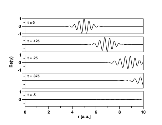
Figure 3: Time evolution of the wave packet described at $t=0$ by Eq. (70); $k_{0}=15$. In the $r$ interval between $0$ and $10$, the potential is constant [$V_{0}=5$ and $a=10$ in Eq. (1)].

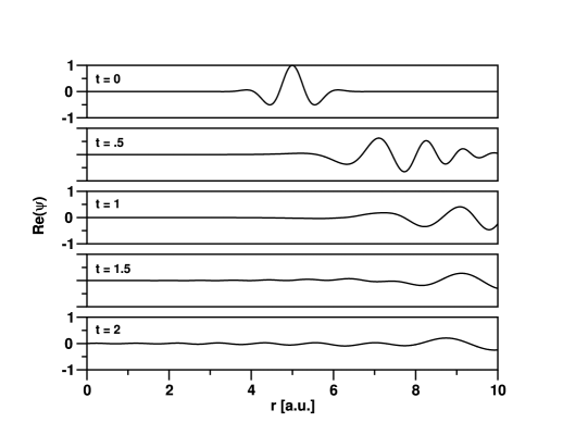
Figure 4: The same parameters as in Fig. 3, but with $k_{0}=5$. Notice that there are significant physical reflections as soon as the wave packet hits the discontinuity at $r=a$.

Table 2: The time-dependent $\chi^{2}$’s discussed in Sec. III for the case of the fast-moving wave packet ($k_{0}=15$; see Fig. 3). $\chi_{3}^{2}(t)$ measures the quality of exponential time evolution, the wave packet being expanded in a basis of bound and outgoing Siegert pseudostates [Eq. (52)]. $\chi_{5}^{2}(t)$ refers to nonexponential time evolution using all $2N$ Siegert pseudostates [Eqs. (62), (69)]. $\parallel\psi(t)\parallel^{2}$ is defined in Eq. (81). The information in this table confirms that both expansions are accurate in describing the motion of a higher-energy particle.

$t$ [a.u.]	$\chi_{3}^{2}(t)/\parallel\psi(t)\parallel^{2}$	$\chi_{5}^{2}(t)/\parallel\psi(t)\parallel^{2}$
$0$	$6.2\times 10^{-14}$	$6.2\times 10^{-14}$
$0.125$	$1.4\times 10^{-13}$	$1.4\times 10^{-13}$
$0.25$	$2.2\times 10^{-13}$	$2.2\times 10^{-13}$
$0.375$	$1.5\times 10^{-12}$	$1.5\times 10^{-12}$
$0.5$	$1.9\times 10^{-9}$	$1.9\times 10^{-9}$

Table 3: The case of the slow-moving wave packet ($k_{0}=5$; see Fig. 4). $\chi_{3}^{2}(t)$ tests Eq. (52); $\chi_{5}^{2}(t)$ tests Eqs. (62) and (69). $\parallel\psi(t)\parallel^{2}$ is defined in Eq. (81). For both forms of expansion coefficients [Eq. (52) vs. Eq. (69)], the accuracy at $t=0$ is only limited by the finite-element basis set. For $t>0$, $\chi_{5}^{2}(t)$ is many orders of magnitude smaller than $\chi_{3}^{2}(t)$, showing that, for this case, accurate time evolution is given by the expansion of Eq. (62) using the nonexponential time-evolution coefficients in Eq. (69).

$t$ [a.u.]	$\chi_{3}^{2}(t)/\parallel\psi(t)\parallel^{2}$	$\chi_{5}^{2}(t)/\parallel\psi(t)\parallel^{2}$
$0$	$2.9\times 10^{-16}$	$2.9\times 10^{-16}$
$0.5$	$6.2\times 10^{-6}$	$5.3\times 10^{-16}$
$1$	$5.5\times 10^{-5}$	$2.2\times 10^{-15}$
$1.5$	$4.4\times 10^{-4}$	$2.4\times 10^{-14}$
$2$	$1.2\times 10^{-3}$	$2.3\times 10^{-13}$

In order to gauge the accuracy of Eq. (52) [i.e., exponential time evolution using a basis of $N$ Siegert pseudostates], we modified $\chi_{3}^{2}$, Eq. (77), to include time dependence. We refer to this straightforward extension as $\chi_{3}^{2}(t)$. An analogous modification of Eq. (80)—$\chi_{5}^{2}(t)$—was introduced to test the nonexponential time evolution expressed by Eqs. (62) and (69). Tables 2 and 3 were calculated with $N=620$. They compare time evolution using Eq. (52) with time evolution given by Eqs. (62) and (69) Faddee . To account for decaying amplitude within the region $[0,a]$, we divide $\chi_{3}^{2}(t)$ and $\chi_{5}^{2}(t)$ by

$$\parallel\psi(t)\parallel^{2}=\int_{0}^{a}\left|\psi(r;t)\right|^{2}\mathrm{d}r\;.$$ (81)

One sees in Table 2 that for the case where $k_{0}=15$, Eq. (52) gives accurate time evolution, while Table 3 shows a significant loss of precision for the slower wave packet, $k_{0}=5$, at all $t>0$. This is because the assumption of pure exponential time evolution in Eq. (52) is not justified. In fact, the more complicated time evolution suggested by Eq. (69) provides superior agreement for both $k_{0}=15$ and $k_{0}=5$. It is important to notice that the expansion coefficients associated with all Siegert pseudostates evolve in time in a nonexponential fashion. [Equation (52) fails also—for $k_{0}=5$—if $V_{0}$ is chosen to be so small that there are no bound states in the well.] Nevertheless, at least when $k_{0}=15$ (and bound and outgoing Siegert pseudostates are selected), Eq. (52) is satisfactory. In this case, we found numerically that the vector defined by its elements ${\bm{c}}_{n}^{\mathrm{T}}{\bm{S}}{\bm{\alpha}}=(\varphi_{n}|\psi)$, $n=1,\ldots,N$, is, to machine precision, an eigenvector of the matrix ${\bm{M}}\in\mathbb{C}^{N\times N}$ with eigenvalue one. As a consequence, the coefficients $\gamma_{n}$ in Eqs. (75) and (77) equal $(\varphi_{n}|\psi)$. This means that Eq. (52) reduces to Eq. (4). We form the conjecture that this is the reason why the approach of Refs. YoWa99 ; TaWa01 , based on Eq. (4), has been successful. [For $k_{0}=5$, we found the performance of Eq. (4) to be even worse than that of Eq. (52).] The most general and accurate treatment, however, is only accomplished on the basis of the time evolution derived from the outgoing-wave Green’s function, Eqs. (62) and (69).

IV Conclusion

In this paper, we reviewed the numerical technique developed by Tolstikhin, Ostrovsky, and Nakamura ToOs97 ; ToOs98 for calculating Siegert pseudostates. The approach is applicable to general short-range potentials; it is not restricted to the simple model potential we made use of in our numerical investigation. We incorporated a straightforward extension of the method to nonorthogonal basis sets and explored in some detail the mathematical properties of the Siegert pseudovectors, in particular questions of completeness.

Our main goal in this paper has been the development of a rigorous formulation of the time evolution of a wave packet expanded in terms of Siegert pseudostates. Our study demonstrates that assuming pure exponential time evolution can be a poor approximation. The technique based on Eqs. (62) and (69), which implies nonexponential time evolution for the entire set of $2N$ Siegert pseudostates, can reproduce very well the analytical reference wave packet moving in the model potential. There are no artificial reflections at the boundary of the grid ($r=a$). Physical reflections are correctly reproduced.

We have shown that it is possible to find a subset consisting of $N$ Siegert pseudovectors that represents a basis of $\mathbb{C}^{N}$. Siegert pseudostates were used in Ref. HaGr02 to carry out channel expansions in the context of multichannel quantum defect theory, using bound and outgoing Siegert pseudostates only. This paper confirms that such a choice provides a complete basis, in principle. In the time domain, this means that a wave packet can be represented for any $t>0$ as a superposition of these $N$ basis states. Their time evolution is, however, nonexponential. The time-dependent expansion coefficients may be found by applying the completeness relation implied by Eq. (51) to the expansion in Eq. (62).

While wave-packet propagation using Eqs. (62) and (69) is numerically stable and accurate, the calculation of all $2N$ eigenvalues and eigenvectors of the generalized eigenvalue problem in Eq. (20) is necessary in principle. This requirement poses a challenge for iterative sparse-matrix techniques. Further developments will be needed in order to turn Siegert pseudostates into a useful tool for large-scale calculations on atoms and molecules. Siegert pseudostates have already offered a glimpse at their extraordinary potential.

Appendix A Existence of a subset of the $2N$ Siegert pseudovectors forming a basis of $\mathbb{C}^{N}$

Let $N_{\mathrm{C}}$ denote the number of eigenvectors ${\bm{c}}_{n}$ whose eigenvalue $\varkappa_{n}$ satisfies $\mathrm{Im}(\varkappa_{n})>0$ [$\mathrm{Re}(k_{n})>0$]. There is an identical number of eigenvectors ${\bm{c}}_{n}$ with $\mathrm{Im}(\varkappa_{n})<0$ [$\mathrm{Re}(k_{n})<0$]. The remaining $2N-2N_{\mathrm{C}}$ eigenvectors are characterized by $\mathrm{Im}(\varkappa_{n})=0$ [$\mathrm{Re}(k_{n})=0$]. The latter correspond to the bound and the antibound states. We order the $2N$ eigenvectors as follows:

$$\underbrace{{\bm{c}}_{1},\ldots,{\bm{c}}_{N_{\mathrm{C}}}}_{\mathrm{Im}(\varkappa_{n})>0},\underbrace{{\bm{c}}_{N_{\mathrm{C}}+1},\ldots,{\bm{c}}_{2N-N_{\mathrm{C}}}}_{\mathrm{Im}(\varkappa_{n})=0},\underbrace{{\bm{c}}_{2N-N_{\mathrm{C}}+1},\ldots,{\bm{c}}_{2N}}_{\mathrm{Im}(\varkappa_{n})<0}\;.$$ (82)

Additionally, the vectors ${\bm{c}}_{2N-N_{\mathrm{C}}+1},\ldots,{\bm{c}}_{2N}$ are ordered in such a way that

$${\bm{c}}_{2N-N_{\mathrm{C}}+n}={\bm{c}}_{n}^{\ast}\;,\;n=1,\ldots,N_{\mathrm{C}}$$ (83)

[note the remarks following Eq. (16)]. We now describe a constructive approach for expressing the last $N_{\mathrm{C}}$ Siegert pseudovectors in Eq. (82) [$\mathrm{Re}(k_{n})<0$] in terms of the vectors ${\bm{c}}_{1},\ldots,{\bm{c}}_{2N-N_{\mathrm{C}}}$.

Equations (39) and (40) can be multiplied from the right by ${\bm{S}}{\bm{c}}_{m}$. Let, in particular, $1\leq m\leq N_{\mathrm{C}}$. Then we can exploit that ${\bm{c}}_{m}^{{\dagger}}{\bm{S}}{\bm{c}}_{m}>0$ and solve for ${\bm{c}}_{m}^{\ast}$:

$${\bm{c}}_{m}^{\ast} = -\sum_{n=1}^{2N-N_{\mathrm{C}}}\frac{\varkappa_{m}^{\ast}}{\varkappa_{n}}\frac{{\bm{c}}_{n}^{\mathrm{T}}{\bm{S}}{\bm{c}}_{m}}{{\bm{c}}_{m}^{{\dagger}}{\bm{S}}{\bm{c}}_{m}}{\bm{c}}_{n}$$

$$-\sum_{n=1(n\neq m)}^{N_{\mathrm{C}}}\frac{\varkappa_{m}^{\ast}}{\varkappa_{n}^{\ast}}\frac{{\bm{c}}_{n}^{{\dagger}}{\bm{S}}{\bm{c}}_{m}}{{\bm{c}}_{m}^{{\dagger}}{\bm{S}}{\bm{c}}_{m}}{\bm{c}}_{n}^{\ast}\;,$$

$${\bm{c}}_{m}^{\ast} = \frac{2}{{\bm{c}}_{m}^{{\dagger}}{\bm{S}}{\bm{c}}_{m}}{\bm{c}}_{m}-\sum_{n=1}^{2N-N_{\mathrm{C}}}\frac{{\bm{c}}_{n}^{\mathrm{T}}{\bm{S}}{\bm{c}}_{m}}{{\bm{c}}_{m}^{{\dagger}}{\bm{S}}{\bm{c}}_{m}}{\bm{c}}_{n}$$ (85)

$$-\sum_{n=1(n\neq m)}^{N_{\mathrm{C}}}\frac{{\bm{c}}_{n}^{{\dagger}}{\bm{S}}{\bm{c}}_{m}}{{\bm{c}}_{m}^{{\dagger}}{\bm{S}}{\bm{c}}_{m}}{\bm{c}}_{n}^{\ast}\;.$$

According to these equations, ${\bm{c}}_{2N}={\bm{c}}_{N_{\mathrm{C}}}^{\ast}$ can be represented in terms of ${\bm{c}}_{1},\ldots,{\bm{c}}_{2N-1}$, i.e.,

$$\mathrm{rank}([{\bm{c}}_{1},\ldots,{\bm{c}}_{2N-1}])=\mathrm{rank}([{\bm{c}}_{1},\ldots,{\bm{c}}_{2N}])=N\;.$$ (86)

Let us assume now that, using Eqs. (A) and (85), we have been able to show for a fixed $m$, $1\leq m\leq N_{\mathrm{C}}$, that

$${\bm{c}}_{N_{\mathrm{C}}-n+1}^{\ast}=\sum_{k=1}^{2N-N_{\mathrm{C}}}\alpha_{k}^{(n)}{\bm{c}}_{k}+\sum_{k=1}^{N_{\mathrm{C}}-m}\beta_{k}^{(n)}{\bm{c}}_{k}^{\ast}\;,\;n=1,\ldots,m$$ (87)

for suitably chosen $\alpha_{k}^{(n)},\beta_{k}^{(n)}\in\mathbb{C}$. This is clearly true for $m=1$ [Eq. (86)]. It follows from Eq. (87) that $\mathrm{rank}({\bm{C}})=N$, where ${\bm{C}}=[{\bm{c}}_{1},\ldots,{\bm{c}}_{2N-m}]$. Also note that the coefficients $\alpha_{k}^{(n)},\beta_{k}^{(n)}$ cannot be unique (since $2N-m>N$), unless $m=N_{\mathrm{C}}$ and $N_{\mathrm{C}}=N$. In fact, there are an infinite number of solutions. This is easy to see: Any solution ${\bm{z}}^{(n)}\in\mathbb{C}^{2N-m}$ of ${\bm{C}}{\bm{z}}^{(n)}={\bm{c}}_{N_{\mathrm{C}}-n+1}^{\ast}$ can be written as the sum of a particular solution of this linear system (which exists, by assumption) and a solution ${\bm{y}}\in\mathbb{C}^{2N-m}$ of the homogeneous system, ${\bm{C}}{\bm{y}}={\bm{0}}$. The kernel of the matrix ${\bm{C}}$ is nontrivial, for its dimension is $\mathrm{dim}(\mathbb{C}^{2N-m})-\mathrm{rank}({\bm{C}})=N-m$. Hence, there are infinitely many vectors ${\bm{y}}$ satisfying the homogeneous system.

We must make the step from $m$ to $m+1$. It is sufficient to demonstrate that

$${\bm{c}}_{N_{\mathrm{C}}-m}^{\ast}=\sum_{k=1}^{2N-N_{\mathrm{C}}}\alpha_{k}^{(m+1)}{\bm{c}}_{k}+\sum_{k=1}^{N_{\mathrm{C}}-m-1}\beta_{k}^{(m+1)}{\bm{c}}_{k}^{\ast}\;.$$ (88)

Equation (A), applied to ${\bm{c}}_{N_{\mathrm{C}}-m}^{\ast}$, can be written as

$${\bm{c}}_{N_{\mathrm{C}}-m}^{\ast} = \sum_{n=1}^{2N-N_{\mathrm{C}}}(\ldots){\bm{c}}_{n}+\sum_{n=1}^{N_{\mathrm{C}}-m-1}(\ldots){\bm{c}}_{n}^{\ast}$$

$$-\sum_{n=N_{\mathrm{C}}-m+1}^{N_{\mathrm{C}}}\frac{\varkappa_{N_{\mathrm{C}}-m}^{\ast}}{\varkappa_{n}^{\ast}}\frac{{\bm{c}}_{n}^{{\dagger}}{\bm{S}}{\bm{c}}_{N_{\mathrm{C}}-m}}{{\bm{c}}_{N_{\mathrm{C}}-m}^{{\dagger}}{\bm{S}}{\bm{c}}_{N_{\mathrm{C}}-m}}{\bm{c}}_{n}^{\ast}\;.$$

Combined with Eq. (87), this yields

$${\bm{c}}_{N_{\mathrm{C}}-m}^{\ast} = \sum_{n=1}^{2N-N_{\mathrm{C}}}(\ldots){\bm{c}}_{n}+\sum_{n=1}^{N_{\mathrm{C}}-m-1}(\ldots){\bm{c}}_{n}^{\ast}$$ (90)

$$-\sum_{n=N_{\mathrm{C}}-m+1}^{N_{\mathrm{C}}}\frac{\varkappa_{N_{\mathrm{C}}-m}^{\ast}}{\varkappa_{n}^{\ast}}\frac{{\bm{c}}_{n}^{{\dagger}}{\bm{S}}{\bm{c}}_{N_{\mathrm{C}}-m}}{{\bm{c}}_{N_{\mathrm{C}}-m}^{{\dagger}}{\bm{S}}{\bm{c}}_{N_{\mathrm{C}}-m}}$$

$$\times\beta_{N_{\mathrm{C}}-m}^{(N_{\mathrm{C}}-n+1)}{\bm{c}}_{N_{\mathrm{C}}-m}^{\ast}\;.$$

The exact form of the coefficients symbolized by $(\ldots)$ is inessential. If we use Eq. (85) in place of Eq. (A), we find

$${\bm{c}}_{N_{\mathrm{C}}-m}^{\ast} = \sum_{n=1}^{2N-N_{\mathrm{C}}}(\ldots){\bm{c}}_{n}+\sum_{n=1}^{N_{\mathrm{C}}-m-1}(\ldots){\bm{c}}_{n}^{\ast}$$ (91)

$$-\sum_{n=N_{\mathrm{C}}-m+1}^{N_{\mathrm{C}}}\frac{{\bm{c}}_{n}^{{\dagger}}{\bm{S}}{\bm{c}}_{N_{\mathrm{C}}-m}}{{\bm{c}}_{N_{\mathrm{C}}-m}^{{\dagger}}{\bm{S}}{\bm{c}}_{N_{\mathrm{C}}-m}\ }$$

$$\times\beta_{N_{\mathrm{C}}-m}^{(N_{\mathrm{C}}-n+1)}{\bm{c}}_{N_{\mathrm{C}}-m}^{\ast}\;.$$

Therefore, as long as either

$$-\sum_{n=N_{\mathrm{C}}-m+1}^{N_{\mathrm{C}}}\frac{\varkappa_{N_{\mathrm{C}}-m}^{\ast}}{\varkappa_{n}^{\ast}}\frac{{\bm{c}}_{n}^{{\dagger}}{\bm{S}}{\bm{c}}_{N_{\mathrm{C}}-m}}{{\bm{c}}_{N_{\mathrm{C}}-m}^{{\dagger}}{\bm{S}}{\bm{c}}_{N_{\mathrm{C}}-m}}\beta_{N_{\mathrm{C}}-m}^{(N_{\mathrm{C}}-n+1)}$$

or

$$-\sum_{n=N_{\mathrm{C}}-m+1}^{N_{\mathrm{C}}}\frac{{\bm{c}}_{n}^{{\dagger}}{\bm{S}}{\bm{c}}_{N_{\mathrm{C}}-m}}{{\bm{c}}_{N_{\mathrm{C}}-m}^{{\dagger}}{\bm{S}}{\bm{c}}_{N_{\mathrm{C}}-m}}\beta_{N_{\mathrm{C}}-m}^{(N_{\mathrm{C}}-n+1)}$$

differ from one, Eq. (88) is satisfied. Otherwise, since the coefficients $\beta_{k}^{(n)}$ are not unique, it is possible in general to choose the $\beta_{N_{\mathrm{C}}-m}^{(N_{\mathrm{C}}-n+1)}$ such that either Eq. (90) or (91) can be solved for ${\bm{c}}_{N_{\mathrm{C}}-m}^{\ast}$.

The coefficients $\beta_{N_{\mathrm{C}}-m}^{(N_{\mathrm{C}}-n+1)}$ will be unique, however, if and only if

$$\mathrm{rank}([{\bm{c}}_{1},\ldots,{\bm{c}}_{2N-m}])=\mathrm{rank}([{\bm{c}}_{1},\ldots,{\bm{c}}_{2N-m-1}])+1\;,$$ (92)

which would also be consistent with the disappearance from Eqs. (90) and (91) of the term involving ${\bm{c}}_{N_{\mathrm{C}}-m}^{\ast}$. Thus, in exact arithmetic, it is conceivable that the construction step from $m$ to $m+1$ fails, i.e., we cannot prove that all incoming Siegert pseudovectors can be eliminated. (Nevertheless, there is no reason to anticipate this to cause any difficulties in numerical calculations.) If really necessary, then the vector ${\bm{c}}_{N_{\mathrm{C}}-m}^{\ast}$ must be kept as an essential basis vector, and the construction procedure outlined above may be continued for the remaining vectors ${\bm{c}}_{1},\ldots,{\bm{c}}_{2N-m-1}$.

Not only the vectors ${\bm{c}}_{n}^{\ast}$ [$\mathrm{Re}(k_{n})<0$] can be eliminated (except for the possible—though unlikely—occurrence of essential vectors), but equations analogous to Eqs. (A) and (85) exist also for the bound and the antibound eigenvectors. Note that for these, ${\bm{c}}_{m}^{\mathrm{T}}{\bm{S}}{\bm{c}}_{m}$ differs from $0$. It is therefore clear that $N$ linearly independent basis vectors ${\bm{c}}_{n}$, $n=1,\ldots,N$, can be found among the vectors ${\bm{c}}_{1},\ldots,{\bm{c}}_{2N}$. The completeness relation satisfied by these $N$ vectors is given by Eq. (51).

Appendix B Time evolution and the Faddeeva function

For evaluating the integral in Eq. (II), it is useful to perform the substitution

$$s^{2}=\mathrm{i}k^{2}t/2\;.$$ (93)

Thus,

$$\int_{-\infty}^{\infty}\frac{\mathrm{e}^{-\mathrm{i}k^{2}t/2}}{k-k_{n}}\mathrm{d}k=\int_{-\sqrt{\mathrm{i}t/2}\infty}^{+\sqrt{\mathrm{i}t/2}\infty}\frac{\mathrm{e}^{-s^{2}}}{s-\sqrt{\mathrm{i}t/2}k_{n}}\mathrm{d}s\;.$$ (94)

The right-hand side of this equation is reminiscent of the Faddeeva function defined in Eq. (68). However, the integration path must be rotated back to the real axis. In order to do this, we must carefully distinguish between poles due to bound, antibound, outgoing, or incoming Siegert pseudostates. The pole of the integrand on the right-hand side of Eq. (94) lies in the upper $s$ plane if, for $t>0$ ($\sqrt{t/2}>0$),

$$\sqrt{\frac{\mathrm{i}t}{2}}=\mathrm{e}^{\mathrm{i}\pi/4}\sqrt{\frac{t}{2}}$$ (95)

for bound or outgoing Siegert pseudostates, and

$$\sqrt{\frac{\mathrm{i}t}{2}}=-\mathrm{e}^{\mathrm{i}\pi/4}\sqrt{\frac{t}{2}}$$ (96)

for antibound or incoming Siegert pseudostates. (Note that the Faddeeva function is defined in the upper half-plane.)

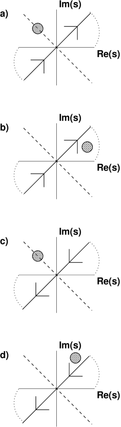
Figure 5: The integration contour used to evaluate Eq. (94) depends on the nature of the Siegert pseudostate considered. Arrows indicate the direction of the integration path in the complex $s$ plane. The circle symbolizes the location of the pole of the integrand on the right-hand side of Eq. (94). a) Bound state. b) Outgoing Siegert pseudostate. c) Antibound state. d) Incoming Siegert pseudostate.

Let us first consider a bound state. In this case, the pole is in the second quadrant of the complex $s$ plane. The integration path, illustrated in Fig. 5a together with the location of the bound-state pole, runs along the diagonal from the third to the first quadrant. Since the contour may be closed as indicated in the figure, and since there are no poles inside the resulting loop, we find

$$\int_{-\sqrt{\mathrm{i}t/2}\infty}^{+\sqrt{\mathrm{i}t/2}\infty}\frac{\mathrm{e}^{-s^{2}}}{s-\sqrt{\mathrm{i}t/2}k_{n}}\mathrm{d}s = \int_{-\infty}^{\infty}\frac{\mathrm{e}^{-s^{2}}}{s-\mathrm{e}^{\mathrm{i}\pi/4}\sqrt{t/2}k_{n}}\mathrm{d}s$$ (97)

$$= -\frac{\pi}{\mathrm{i}}w\left(\mathrm{e}^{\mathrm{i}\pi/4}\sqrt{\frac{t}{2}}k_{n}\right)$$

for a bound state.

The location of the pole in the case of an outgoing Siegert pseudostate is shown in Fig. 5b. This time the pole lies inside the integration loop, so that

$$\int_{-\sqrt{\mathrm{i}t/2}\infty}^{+\sqrt{\mathrm{i}t/2}\infty}\frac{\mathrm{e}^{-s^{2}}}{s-\sqrt{\mathrm{i}t/2}k_{n}}\mathrm{d}s = -2\pi\mathrm{i}\mathrm{e}^{-\mathrm{i}k_{n}^{2}t/2}$$

$$-\frac{\pi}{\mathrm{i}}w\left(\mathrm{e}^{\mathrm{i}\pi/4}\sqrt{\frac{t}{2}}k_{n}\right)$$

for an outgoing Siegert pseudostate.

The pole’s location for an antibound and an incoming Siegert pseudostate, respectively, can be seen in Figs. 5c and 5d. (The integration path now runs along the diagonal from the first to the third quadrant.) In neither case does the pole interfere with the rotation of the integration path to the real $s$ axis. Therefore, for an antibound or incoming Siegert pseudostate the result reads

$$\int_{-\sqrt{\mathrm{i}t/2}\infty}^{+\sqrt{\mathrm{i}t/2}\infty}\frac{\mathrm{e}^{-s^{2}}}{s-\sqrt{\mathrm{i}t/2}k_{n}}\mathrm{d}s = -\int_{-\infty}^{\infty}\frac{\mathrm{e}^{-s^{2}}}{s+\mathrm{e}^{\mathrm{i}\pi/4}\sqrt{t/2}k_{n}}\mathrm{d}s$$ (99)

$$= \frac{\pi}{\mathrm{i}}w\left(-\mathrm{e}^{\mathrm{i}\pi/4}\sqrt{\frac{t}{2}}k_{n}\right)\;.$$

References

- (1) A. J. F. Siegert, Phys. Rev. 56, 750 (1939).
- (2) H. J. Korsch, R. Möhlenkamp, and H.-D. Meyer, J. Phys. B 17, 2955 (1984).
- (3) R. G. Newton, Scattering Theory of Waves and Particles (Dover, Mineola, N.Y., 2002).
- (4) R. M. More and E. Gerjuoy, Phys. Rev. A 7, 1288 (1973).
- (5) O. I. Tolstikhin, V. N. Ostrovsky, and H. Nakamura, Phys. Rev. Lett. 79, 2026 (1997).
- (6) O. I. Tolstikhin, V. N. Ostrovsky, and H. Nakamura, Phys. Rev. A 58, 2077 (1998).
- (7) W. P. Reinhardt, Ann. Rev. Phys. Chem. 33, 223 (1982).
- (8) N. Moiseyev, Phys. Rep. 302, 211 (1998).
- (9) T. N. Rescigno, C. W. McCurdy, Jr., and A. E. Orel, Phys. Rev. A 17, 1931 (1978).
- (10) R. Santra and L. S. Cederbaum, Phys. Rep. 368, 1 (2002).
- (11) U. V. Riss and H.-D. Meyer, J. Phys. B 26, 4503 (1993).
- (12) J. N. Bardsley and B. R. Junker, J. Phys. B 5, L178 (1972).
- (13) C. W. McCurdy and T. N. Rescigno, Phys. Rev. A 20, 2346 (1979).
- (14) B. I. Schneider, Phys. Rev. A 24, 1 (1981).
- (15) E. L. Hamilton and C. H. Greene, Phys. Rev. Lett. 89, 263003 (2002).
- (16) S. Yoshida, S. Watanabe, C. O. Reinhold, and J. Burgdörfer, Phys. Rev. A 60, 1113 (1999).
- (17) S. Tanabe, S. Watanabe, N. Sato, M. Matsuzawa, S. Yoshida, C. Reinhold, and J. Burgdörfer, Phys. Rev. A 63, 052721 (2001).
- (18) R. Narasimhan and Y. Nievergelt, Complex Analysis in One Variable (Birkhäuser, Boston, 2001).
- (19) M. L. Goldberger and K. M. Watson, Collision Theory (Wiley, New York, 1964). Equation (40d) on page 434 of this reference, which corresponds to our Eq. (62), contains a sign error.
- (20) V. N. Faddeeva and N. M. Terent’ev, Tables of Values of the Function for Complex Argument (Pergamon, Oxford, 1961).
- (21) B. D. Fried and S. D. Conte, The Plasma Dispersion Function (Academic, New York, 1961).
- (22) J. Humlíček, J. Quant. Spectrosc. Ra. 21, 309 (1979).
- (23) G. Németh, Á. Ág, and Gy. Páris, J. Math. Phys. 22, 1192 (1981).
- (24) G. P. M. Poppe and C. M. J. Wijers, ACM Trans. Math. Software 16, 38 (1990).
- (25) D. Summers and R. M. Thorne, Phys. Fluids B 3, 1835 (1991).
- (26) R. J. Wells, J. Quant. Spectrosc. Ra. 62, 29 (1999).
- (27) K. J. Bathe, Finite Element Procedures in Engineering Analysis (Prentice Hall, Englewood Cliffs, NJ, 1976).
- (28) K. J. Bathe and E. Wilson, Numerical Methods in Finite Element Analysis (Prentice Hall, Englewood Cliffs, NJ, 1976).
- (29) M. Braun, W. Schweizer, and H. Herold, Phys. Rev. A 48, 1916 (1993).
- (30) J. Ackermann and J. Shertzer, Phys. Rev. A 54, 365 (1996).
- (31) T. N. Rescigno, M. Baertschy, D. Byrum, and C. W. McCurdy, Phys. Rev. A 55, 4253 (1997).
- (32) K. W. Meyer, C. H. Greene, and B. D. Esry, Phys. Rev. Lett. 78, 4902 (1997).
- (33) R. Santra, K. V. Christ, and C. H. Greene, Phys. Rev. A 69, 042510 (2004).
- (34) E. Anderson, Z. Bai, C. Bischof, S. Blackford, J. Demmel, J. Dongarra, J. Du Croz, A. Greenbaum, S. Hammarling, A. McKenney, and D. Sorensen, LAPACK Users’ Guide (Society for Industrial and Applied Mathematics, Philadelphia, 1999).
- (35) M. Abramowitz and I. A. Stegun (Eds.), Handbook of Mathematical Functions (Dover, New York, 1970).
- (36) R. Jacob and R. G. Sachs, Phys. Rev. 121, 350 (1961).
- (37) R. G. Winter, Phys. Rev. 123, 1503 (1961).
- (38) D. A. Dicus, W. W. Repko, R. F. Schwitters, and T. M. Tinsley, Phys. Rev. A 65, 032116 (2002).
- (39) C. A. Nicolaides and D. R. Beck, Phys. Rev. Lett. 38, 683 (1977).
- (40) C. A. Nicolaides, Phys. Rev. A 66, 022118 (2002).
- (41) The Faddeeva function in Eq. (69) was numerically evaluated using the algorithm described in Ref. PoWi90 .