The novel aspect of hydrogen atom: the fine structure and spin can be derived by single component wavefunction

Abstract

The fine structure of hydrogen energy was calculated by using the usual momentum-wavefunction relation directly, rather than establishing the well-known Dirac wave equation. As the results, the energy levels are completely the same as that of the Dirac wave equation, while the wavefunction is single component that is quite different from Dirac’s four component wavefunction, the most important thing is that the present calculation brings out electronic spin in a new way which has never been reported and indicates that the electronic spin is a kind of orbital motion.
PACS numbers: 03.65Bz, 32.10.Fn

1 Introduction

As we know, the fine structure and electronic spin in hydrogen atom can be exactly calculated by using the Dirac wave equation which contains four component wavefunction, the work is a milestone in physics. Up to now, it has been believed that electronic spin must be theocretically specified by Dirac’s four component wavefunction, spin concept has been developed as one of the most important properties of elementary particles in high energy physics.

Consider a particle of rest mass $m$ and charge $q$ moving in an inertial frame of reference with relativistic 4-vector velocity $u_{\mu}$, it satisfies[1]

$$u_{\mu}u_{\mu}=-c^{2}$$ (1)

where there is not distinction between covariant and contravariant components in the Cartesian coordinate system. Eq.(1) is just the relativistic energy-momentum relation when multiplying it by squared mass. Let $A_{\mu}$ denote vector potential of electromagnetic field, substituting the momentum-wavefunction relation[2]

$$mu_{\mu}=\frac{1}{\psi}(-i\hbar\partial_{\mu}-qA_{\mu})\psi$$ (2)

into Eq.(1), we obtain a new quantum wave equation with single component wavefunction

$$[(-i\hbar\partial_{\mu}-qA_{\mu})\psi][(-i\hbar\partial_{\mu}-qA_{\mu})\psi]=-m^{2}c^{2}\psi^{2}$$ (3)

Note that taking the right side of Eq.(2) as momentum-operator to replace momentum that appears in a physical equation is a traditional usage, but in this paper we directly use the right side of Eq.(2) as momentum as we have done in Eq.(3). Please note that Eq.(3) is not the Klein-Gordon wave equation.

In the recent years, H. Y. Cui[3, 4] has reported some significant results of Eq.(3) for certain physical systems. In this paper I point out that the fine structure of hydrogen energy can also be calculated by using Eq.(3), while its wavefunction has single component in contrast with Dirac’s wavefunction, the spin effect of electron is also revealed by Eq.(3) when the hydrogen atom is in a magnetic field, the present calculation totally does not need multi-component wavefunction for specifying electronic spin, and indicates that we should re-recognize spin.

2 The fine structure of hydrogen energy

In the following, we use Gaussian units, and use $m_{e}$ to denote the rest mass of electron.

In a spherical polar coordinate system $(r,\theta,\varphi,ict)$, the nucleus of hydrogen atom provides a spherically symmetric potential $V(r)=e/r$ for the electron motion. The wave equation (3) for the hydrogen atom in the energy eigenstate $\psi(r,\theta,\varphi)e^{-iEt/\hbar}$ may be written in the spherical coordinates:

$$\frac{m_{e}^{2}c^{2}}{\hbar^{2}}\psi^{2}=(\frac{\partial\psi}{\partial r})^{2}+(\frac{1}{r}\frac{\partial\psi}{\partial\theta})^{2}+(\frac{1}{r\sin\theta}\frac{\partial\psi}{\partial\varphi})^{2}+\frac{1}{\hbar^{2}c^{2}}(E+\frac{e^{2}}{r})^{2}\psi^{2}\\$$

By substituting $\psi=R(r)X(\theta)\phi(\varphi)$, we separate the above equation into

$$(\frac{\partial\phi}{\partial\varphi})^{2}+\kappa\phi^{2} = 0$$

$$(\frac{\partial X}{\partial\theta})^{2}+[\lambda-\frac{\kappa}{\sin^{2}\theta}]X^{2} = 0$$

$$(\frac{\partial R}{\partial r})^{2}+[\frac{1}{\hbar^{2}c^{2}}(E+\frac{e^{2}}{r})^{2}-\frac{m_{e}^{2}c^{2}}{\hbar^{2}}-\frac{\lambda}{r^{2}}]R^{2} = 0$$

where $\kappa$ and $\lambda$ are constants introduced for the separation. Eq.(LABEL:s5) can be solved immediately, with the requirement that $\phi(\varphi)$ must be a periodic function, we find its solution given by

$$\phi=C_{1}e^{\pm i\sqrt{\kappa}\varphi}=C_{1}e^{im\varphi}\qquad m=\pm\sqrt{\kappa}=0,\pm 1,...$$ (7)

where $C_{1}$ is an integral constant.

It is easy to find the solution of Eq.(LABEL:s6), it is given by

$$X(\theta)=C_{2}e^{\pm i\int\sqrt{\lambda-\frac{m^{2}}{\sin^{2}\theta}}d\theta}$$ (8)

where $C_{2}$ is an integral constant. The requirement of periodic function for $X$ demands

$$\int\nolimits_{0}^{2\pi}\sqrt{\lambda-\frac{m^{2}}{\sin^{2}\theta}}d\theta=2\pi k\qquad k=0,1,2,...$$ (9)

This complex integration is evaluated (see the appendix for the details), we get

$$\int\nolimits_{0}^{2\pi}\sqrt{\lambda-\frac{m^{2}}{\sin^{2}\theta}}d\theta=2\pi(\sqrt{\lambda}-|m|)$$ (10)

thus, we obtain

$$\sqrt{\lambda}=k+|m|$$ (11)

We rename the integer $\lambda$ as $j^{2}$ for a convenience in the following, i.e. $\lambda=j^{2}$.

The solution of Eq.(LABEL:s7) is given by

$$R(r)=C_{3}e^{\pm\frac{i}{\hbar c}\int\sqrt{(E+\frac{e^{2}}{r})^{2}-m_{e}^{2}c^{4}-\frac{\lambda\hbar^{2}c^{2}}{r^{2}}}dr}$$ (12)

where $C_{3}$ is an integral constant. The requirement that the radical wavefunction forms a ”standing wave” in the range from $r=0$ to $r=\infty$ demands

$$\frac{1}{\hbar c}\int\nolimits_{0}^{\infty}\sqrt{(E+\frac{e^{2}}{r})^{2}-m_{e}^{2}c^{4}-\frac{\lambda\hbar^{2}c^{2}}{r^{2}}}dr=\pi s$$

$$s=0,1,2,...$$ (13)

This complex integration is evaluated (see the appendix for the details), we get

$$\frac{1}{\hbar c}\int\nolimits_{0}^{\infty}\sqrt{(E+\frac{e^{2}}{r})^{2}-m_{e}^{2}c^{4}-\frac{j^{2}\hbar^{2}c^{2}}{r^{2}}}dr$$

$$=\frac{\pi E\alpha}{\sqrt{m_{e}^{2}c^{4}-E^{2}}}-\pi\sqrt{j^{2}-\alpha^{2}}$$ (14)

where $\alpha=e^{2}/\hbar c$ is known as the fine structure constant.

Form the last Eq.(13) and Eq.(14), we obtain the energy levels given by

$$E=m_{e}c^{2}\left[1+\frac{\alpha^{2}}{(\sqrt{j^{2}-\alpha^{2}}+s)^{2}}\right]^{-\frac{1}{2}}$$ (15)

where $j=\sqrt{\lambda}=k+|m|$. Because $j\neq 0$ in Eq.(15), we find $j=1,2,3...$.

The result, Eq.(15), is completely the same as that in the calculation of the Dirac wave equation[6] for the hydrogen atom, it is just the fine structure of hydrogen energy.

3 The electronic spin

If we put the hydrogen atom into an external uniform magnetic field $B$ which is along the $z$ axis with the vector potential $(A_{r},A_{\theta},A_{\varphi})=(0,0,\frac{1}{2}r\sin\theta B)$, then according to Eq.(3) the wave equation is given by

$$\frac{m_{e}^{2}c^{2}}{\hbar^{2}}\psi^{2} = (\frac{\partial\psi}{\partial r})^{2}+(\frac{1}{r}\frac{\partial\psi}{\partial\theta})^{2}+\frac{1}{\hbar^{2}c^{2}}(E+\frac{e^{2}}{r})^{2}\psi^{2}$$ (16)

$$+(\frac{1}{r\sin\theta}\frac{\partial\psi}{\partial\varphi}-\frac{er\sin\theta B}{i2c\hbar}\psi)^{2}$$

By substituting $\psi=R(r)X(\theta)\phi(\varphi)$, we separate the above equation into

$$\frac{\partial\phi}{\partial\varphi}+\kappa\phi = 0$$

(17)

$$(\frac{\partial X}{\partial\theta})^{2}+[(\frac{-\kappa}{\sin\theta}-\frac{e\sin\theta r^{2}B}{i2c\hbar})^{2}+\xi(r)]X^{2} = 0$$

$$(\frac{\partial R}{\partial r})^{2}+[\frac{1}{\hbar^{2}c^{2}}(E+\frac{e^{2}}{r})^{2}-\frac{m_{e}^{2}c^{2}}{\hbar^{2}}-\frac{\xi(r)}{r^{2}}]R^{2} = 0$$

where we have used the unknown constant $\kappa$ and function $\xi(r)$ to connect these separated equations. Eq.(17) has the solution

$$\phi=C_{1}e^{im\varphi},\qquad\kappa=im,\qquad m=0,\pm 1,\pm 2,...$$ (20)

Expanding Eq.(LABEL:d3) and neglecting the term $O(B^{2})$, we find a constant term $-\frac{mer^{2}B}{c\hbar}$ in it, by moving this term into Eq.(LABEL:d4) through $\xi(r)=\lambda+\frac{mer^{2}B}{c\hbar}$, we obtain

$$(\frac{\partial X}{\partial\theta})^{2}+[\lambda-\frac{m^{2}}{\sin^{2}\theta}]X^{2} = 0$$

$$(\frac{\partial R}{\partial r})^{2}+[\frac{1}{\hbar^{2}c^{2}}(E+\frac{e^{2}}{r})^{2}-\frac{m_{e}^{2}c^{2}}{\hbar^{2}}-\frac{meB}{c\hbar}-\frac{\lambda}{r^{2}}]R^{2} = 0$$

The above two equations are the same as Eq.(LABEL:s6) and Eq.(LABEL:s7), except for the additional constant term $-meB/c\hbar$. After the similar calculation as the preceding section, we obtain the energy levels of hydrogen atom in the magnetic field given by

$$E=\sqrt{m_{e}^{2}c^{4}+mec\hbar B}\left[1+\frac{\alpha^{2}}{(\sqrt{j^{2}-\alpha^{2}}+s)^{2}}\right]^{-\frac{1}{2}}$$ (23)

In the usual spectroscopic notation of quantum mechanics, four quantum numbers: $n$, $l$, $m_{l}$ and $m_{s}$ are used to specify the state of an electron in an atom. After the comparison, we get the relations between the usual notation and our notation.

$$n = j+s,\quad s=0,1,...;j=1,2,....$$ (24)

$$l = j-1,$$ (25)

$$\quad\max(m_{l}) = \max(m)-1$$ (26)

We find that $j$ takes over $1,2,...,n$; for a fixed $j$ (or $l$), $m$ takes over $-(l+1),-l,...,0,...,l,l+1$. In the present work, spin quantum number is absent.

According to Eq.(23), for a fixed $(n,l)$, equivalent to $(n,j=l+1)$, the energy level of hydrogen atom will split into $2l+3$ energy levels in the magnetic field, given by

$$E=(m_{e}c^{2}+\frac{me\hbar B}{2m_{e}c})\left[1+\frac{\alpha^{2}}{(\sqrt{j^{2}-\alpha^{2}}+s)^{2}}\right]^{-\frac{1}{2}}+O(B^{2})\\$$

Considering $m=-(l+1),-l,...,0,...,l,l+1$, this effect is equivalent to the usual Zeeman splitting in the usual quantum mechanics given by

$$E=E_{nl}+\frac{(m_{l}\pm 1)e\hbar B}{2m_{e}c}$$ (27)

But our work works on it without spin concept, the so-called spin effect has been revealed by Eq.(3) without spin concept, this result indicates that electronic spin is a kind of orbital motion.

In Stern-Gerlach experiment, the angular momentum of ground state of hydrogen atom is presumed to be zero according to the usual quantum mechanics, thus ones need make use of the spin. But in the present calculation, the so-called spin has been merged with the orbital motion of the electron.

Recalling that the spin is a mysterious concept even for very learned persons, we have come to this point: we can understand the quantum mechanics without the well-established spin concept, can’t we? without multi-component wavefunction, can’t we? Bear in mind that simplicity is always a merit for the physics.

4 Conclusion

Using equations

$$(mu_{\mu}+qA_{\mu})\psi = -i\hbar\partial_{\mu}\psi$$ (28)

$$u_{\mu}u_{\mu} = -c^{2}$$ (29)

by eliminating $u_{\mu}$, the above equations can be written as

$$-m^{2}c^{2}\psi^{2}=[(-i\hbar\partial_{\mu}-qA_{\mu})\psi][(-i\hbar\partial_{\mu}-qA_{\mu})\psi]$$ (30)

Using this quantum wave equation, the fine structure of hydrogen atom energy is calculated, as the results, the energy levels are given by

$$E = m_{e}c^{2}\left[1+\frac{\alpha^{2}}{(\sqrt{j^{2}-\alpha^{2}}+n)^{2}}\right]^{-\frac{1}{2}}$$ (31)

$$j = 1,2,...;n=0,1,...$$

the result is completely the same as that in the calculation of the Dirac wave equation for the hydrogen atom, while the wavefunction is quite different from Dirac’s wavefunction. Besides, the present calculation brings out spin nature in a new way, indicating that electronic spin is a kind of orbital motion. The present calculation is characterized by using the usual momentum-wavefunction relation directly, it provides an insight into the foundations of quantum mechanics.

Appendix A Appendix: The evaluations of the integrations

In this appendix we give out the evaluations of the integrations appeared in the preceding section, i.e.Eq.(10) and Eq.(14).

A.1 wave-attenuating boundary condition

Consider the integrand in Eq.(10), it is a multiple-valued function, may be written as

$$\sqrt{\lambda-\frac{m^{2}}{\sin^{2}\theta}}=\sqrt{f(\theta)}\qquad f(\theta)=\lambda-\frac{m^{2}}{\sin^{2}\theta}$$ (32)

Suppose that $\lambda$ is a real positive number, the function $f(\theta)$ may be divided into the three regions: $(0,a)$, $(a,b)$, and $(b,\pi)$, where $a$ and $b$ are the turning points at where the function $f(\theta)$ changes its sign, as shown in Fig.1. we find

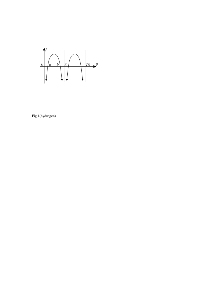
Figure 1: The function has sign-changed points $a$ and $b$.

$$\int\nolimits_{0}^{a}\sqrt{f(\theta)}d\theta = \int\nolimits_{0}^{a}\sqrt{-|f(\theta)|}d\theta=\pm i\int\nolimits_{0}^{a}\sqrt{|f(\theta)|}d\theta$$ (33)

$$= \pm iA$$

$$\int\nolimits_{a}^{b}\sqrt{f(\theta)}d\theta = \int\nolimits_{a}^{b}\sqrt{|f(\theta)|}d\theta=B$$

$$\int\nolimits_{b}^{\pi}\sqrt{f(\theta)}d\theta = \int\nolimits_{b}^{\pi}\sqrt{-|f(\theta)|}d\theta=\pm iA$$

where $A$ and $B$ are two real numbers, then the integration of Eq.(10) has three possible solutions given by

$$\int\nolimits_{0}^{2\pi}\sqrt{\lambda-\frac{m^{2}}{\sin^{2}\theta}}d\theta=\left\{\begin{array}[]{l}2(B+2iA)\\ 2B\\ 2(B-2iA)\end{array}\right.$$ (36)

The second branch of this result is reasonable, because only it can fulfil the requirement that the wavefunction is periodic function of $\theta$. The multiple-valued result arises from that $\sqrt{-|f(\theta)|}=\pm i\sqrt{|f(\theta)|}$, like $\sqrt{-5}=\pm i\sqrt{5}$.

How to determine the sign of the multiple-valued function reasonably? Let us turn to our experience that we have had in the usual quantum mechanics. Consider the motion of a particle in a finitely deep potential well as shown in Fig.2, there are also two turning points $a$ and $b$. If the particle moves over the turning point $a$ or $b$ for $E<V_{0}$ (bound states), its momentum will become imaginary $\pm i|p|$ with uncertain sign. As we know in the usual quantum mechanics the wavefunction is given by

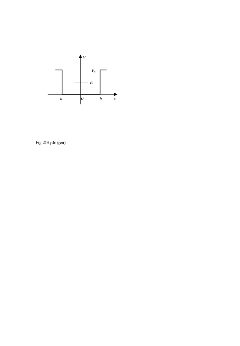
Figure 2: A finitely deep potential well that has two turning points $a$ and $b$.

$$\psi(x)=\left\{\begin{array}[]{ll}De^{-i\frac{i|p|}{\hbar}x}&x<a\\ G\sin(\frac{|p_{{}_{0}}|}{\hbar}x+\delta)&a<x<b\\ De^{-i\frac{-i|p|}{\hbar}x}&x>b\end{array}\right.$$ (37)

This has involved our experience in which we have taken plus sign for the imaginary momentum in $x<a$ and minus sign in $x>b$, to satisfy the so-called wave-attenuating boundary condition for the regions over the turning points.

In the followings, we use this wave-attenuating boundary condition to determine the sign of double-valued imaginary momentum: take plus sign in the region over the left turning point, whereas take minus sign in the region over the right turning point.

A.2 integration 1

To apply the wave-attenuating boundary condition to the following wavefunction

$$X(\theta)=C_{2}e^{-i\int\sqrt{\lambda-\frac{m^{2}}{\sin^{2}\theta}}d\theta}$$ (38)

due to wave-attenuating for the turning points, the integrand must choose the signs as

$$\int\nolimits_{0}^{a}\sqrt{\lambda-\frac{m^{2}}{\sin^{2}\theta}}d\theta = +i\int\nolimits_{0}^{a}\sqrt{|f(\theta)|}d\theta=iA$$ (39)

$$\int\nolimits_{a}^{b}\sqrt{\lambda-\frac{m^{2}}{\sin^{2}\theta}}d\theta = \int\nolimits_{a}^{b}\sqrt{f(\theta)}d\theta=B$$ (40)

$$\int\nolimits_{b}^{\pi}\sqrt{\lambda-\frac{m^{2}}{\sin^{2}\theta}}d\theta = -i\int\nolimits_{b}^{\pi}\sqrt{|f(\theta)|}d\theta=-iA$$ (41)

thus the integration may have a real solution, actually it may be written as

$$\int\nolimits_{0}^{2\pi}\sqrt{\lambda-\frac{m^{2}}{\sin^{2}\theta}}d\theta=2\int\nolimits_{a}^{b}\sqrt{\lambda-\frac{m^{2}}{\sin^{2}\theta}}d\theta=2B$$ (42)

In order to evaluate the definite integral of Eq.(42), we make use of contour integral in complex plane[5]. Consider a contour $C_{\delta}$ which is a unit circle around zero, as shown in Fig.3, using $z=e^{i\theta}$, we have

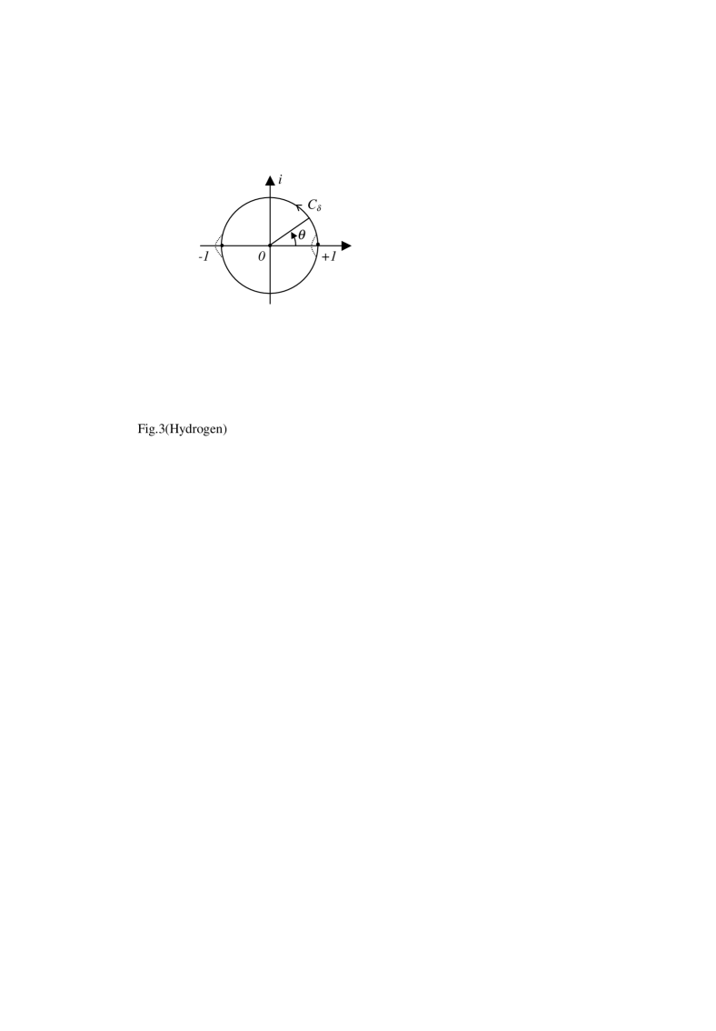
Figure 3: Unit circle contour for evaluating integral

$$I_{1} = \int\nolimits_{0}^{2\pi}\sqrt{\lambda-\frac{m^{2}}{\sin^{2}\theta}}d\theta=\int\nolimits_{C_{\delta}}\sqrt{\lambda+\frac{4m^{2}z^{2}}{(z^{2}-1)^{2}}}\frac{dz}{iz}$$ (43)

$$= \int\nolimits_{C_{\delta}}\frac{\sqrt{\lambda(z^{2}-1)^{2}+4m^{2}z^{2}}}{\pm(z^{2}-1)}\frac{dz}{iz}$$

As we have known that $\sqrt{f(\theta)}|_{\theta=\pi/2,or\theta=3\pi/2}=\sqrt{\lambda-m^{2}}$, substituting $z=i$ or $z=-i$ into the above integrand, we find the integrand must take the minus sign. Thus

$$I_{1}=\int\nolimits_{C_{\delta}}\frac{\sqrt{\lambda(z^{2}-1)^{2}+4m^{2}z^{2}}}{-(z^{2}-1)}\frac{dz}{iz}$$ (44)

For scrutinizing the sign of the integrand over the turning points, we have

$$\sqrt{f(\theta)} = \frac{\sqrt{\lambda(z^{2}-1)^{2}+4m^{2}z^{2}}}{-(z^{2}-1)}$$ (45)

$$= \frac{\sqrt{\lambda(z^{2}-1)^{2}+4m^{2}z^{2}}}{-(2iz)(z^{2}-1)/(2iz)}$$

$$= \frac{\sqrt{\lambda(z^{2}-1)^{2}+4m^{2}z^{2}}}{-(2iz)\sin\theta}$$

$$= i\frac{\sqrt{\lambda(z^{2}-1)^{2}+4m^{2}z^{2}}}{2z\sin\theta}$$

we find that the integrand takes plus sign over the left turning point $(\theta\rightarrow 0+,z\rightarrow 1)$ and minus sign over the right turning point $(\theta\rightarrow\pi-,z\rightarrow-1)$, in accordance with the sign requirement of Eq.(39) and (41).

Continue our calculation, we have

$$I_{1} = \int\nolimits_{C_{\delta}}\frac{\sqrt{\lambda(z^{2}-1)^{2}+4m^{2}z^{2}}}{-(z^{2}-1)}\frac{dz}{iz}$$

$$= \int\nolimits_{C_{\delta}}(\frac{1}{z}-\frac{1/2}{z-1}-\frac{1/2}{z+1})\sqrt{\lambda(z^{2}-1)^{2}+4m^{2}z^{2}}\frac{dz}{i}$$

Now we find that the integrand has the poles at $z=0$ and $z=\pm 1$. We let the counter $C_{\delta}$ pass by the pole $z=+1$ through the interior of the unite circle, as indicated by the dash line in Fig.3, likewise, let the counter $C_{\delta}$ pass by the pole $z=-1$ through the exterior of the unite circle. The deformation made for $C_{\delta}$ has no influence on the integration value because the left deformation cancels the right deformation in the integration due to the opposite signs of the integrand near the left and right poles. Let $C_{\delta}^{\prime}$ denote the deformed counter, we continue the calculation by using residue theorem.

$$I_{1} = \int\nolimits_{C_{\delta}^{\prime}}(\frac{1}{z}-\frac{1/2}{z-1}-\frac{1/2}{z+1})\sqrt{\lambda(z^{2}-1)^{2}+4m^{2}z^{2}}\frac{dz}{i}$$ (47)

$$= \int\nolimits_{C_{\delta}^{\prime}}\frac{1}{z}\sqrt{\lambda(z^{2}-1)^{2}+4m^{2}z^{2}}\frac{dz}{i}$$

$$-\int\nolimits_{C_{\delta}^{\prime}}\frac{1/2}{z-1}\sqrt{\lambda(z^{2}-1)^{2}+4m^{2}z^{2}}\frac{dz}{i}$$

$$-\int\nolimits_{C_{\delta}^{\prime}}\frac{1/2}{z+1}\sqrt{\lambda(z^{2}-1)^{2}+4m^{2}z^{2}}\frac{dz}{i}$$

$$= \int\nolimits_{C_{\delta}^{\prime}}\frac{\sqrt{\lambda}+O(z^{2})}{z}\frac{dz}{i}-\int\nolimits_{C_{\delta}^{\prime}}\frac{|m|+O(z^{2}-1)}{z+1}\frac{dz}{i}$$

$$= 2\pi(\sqrt{\lambda}-|m|)$$

A.3 Integration 2

To apply the wave-attenuating boundary condition to the following wavefunction

$$R(r)=C_{3}e^{-\frac{i}{\hbar c}\int\sqrt{(E+\frac{e^{2}}{r})^{2}-m_{e}^{2}c^{4}-\frac{\lambda\hbar^{2}c^{2}}{r^{2}}}dr}$$ (48)

where it has also two turning points $x$ and $y$ from $r=0$ to $r=\infty$ when $E^{2}<m_{e}^{2}c^{4}$ (bound states), as shown in Fig.4 where

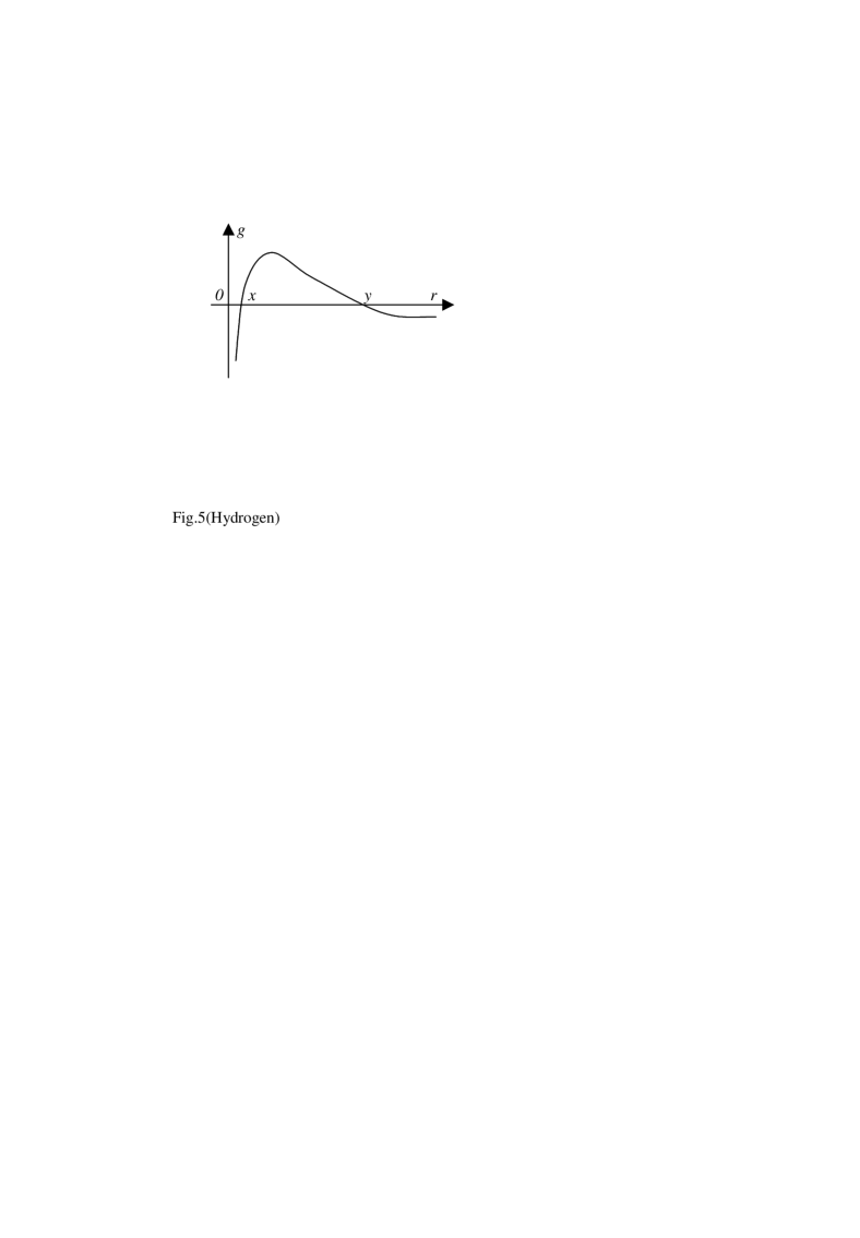
Figure 4: Contour for evaluating integral.

$$g(r)=(E+\frac{e^{2}}{r})^{2}-m_{e}^{2}c^{4}-\frac{j^{2}\hbar^{2}c^{2}}{r^{2}}$$ (49)

we take the following signs for its asymptotic behavior, i.e.

$$\sqrt{g(r)}|_{r\rightarrow 0} = \sqrt{e^{4}-j^{2}\hbar^{2}c^{2}}/r=i\sqrt{j^{2}\hbar^{2}c^{2}-e^{4}}/r$$

$$\sqrt{g(r)}|_{r\rightarrow\infty} = \sqrt{E^{2}-m_{e}^{2}c^{4}}=-i\sqrt{m_{e}^{2}c^{4}-E^{2}}$$

In order to evaluate the definite integral of Eq.(14), consider a contour $C$ consisting of $C_{\gamma}$, $L_{-}$, $C_{\delta}$ and $L$ around zero in the plane as shown in Fig.5, the radius of circle $C_{\gamma}$ is large enough and the radius of circle $C_{\delta}$ is small enough. The integrand of the following equation has no pole inside the contour $C$, so that we have

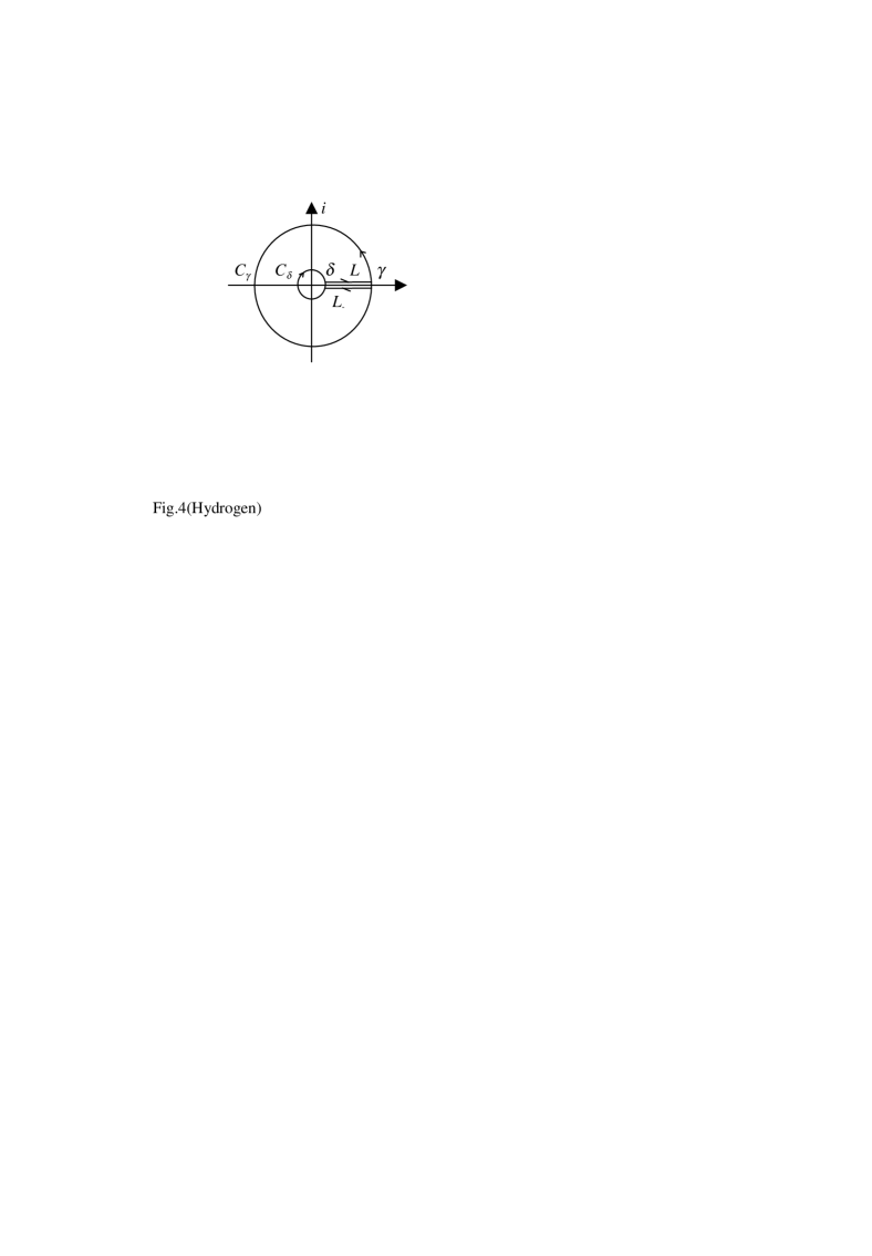
Figure 5: The function has two sign-changed points $x$ and $y$.

$$\int\nolimits_{C}\sqrt{(E+\frac{e^{2}}{z})^{2}-m_{e}^{2}c^{4}-\frac{j^{2}\hbar^{2}c^{2}}{z^{2}}}dz=$$

$$\int\nolimits_{C_{\gamma}}+\int\nolimits_{L_{-}}+\int\nolimits_{C_{\delta}}+\int\nolimits_{L}=0$$ (52)

Now we evaluate the integration on each contour with our sign choice for the double-valued function.

$$\int\nolimits_{C_{\gamma}} = \int\nolimits_{C_{\gamma}}\sqrt{(E+\frac{e^{2}}{z})^{2}-m_{e}^{2}c^{4}-\frac{j^{2}\hbar^{2}c^{2}}{z^{2}}}dz$$ (53)

$$= -\int\nolimits_{C_{\gamma}}i\sqrt{m_{e}^{2}c^{4}+\frac{j^{2}\hbar^{2}c^{2}}{z^{2}}-(E+\frac{e^{2}}{z})^{2}}dz$$

$$= -i\int\nolimits_{C_{\gamma}}[\sqrt{m_{e}^{2}c^{4}-E^{2}}-\frac{Ee^{2}}{\sqrt{m_{e}^{2}c^{4}-E^{2}}}\frac{1}{z}+O(\frac{1}{z^{2}})]dz$$

$$= i\frac{2\pi iEe^{2}}{\sqrt{m_{e}^{2}c^{4}-E^{2}}}=-\frac{2\pi Ee^{2}}{\sqrt{m_{e}^{2}c^{4}-E^{2}}}$$

$$\int\nolimits_{C_{\delta}} = \int\nolimits_{C_{\delta}}i\sqrt{m_{e}^{2}c^{4}+\frac{j^{2}\hbar^{2}c^{2}}{z^{2}}-(E+\frac{e^{2}}{z})^{2}}dz$$ (54)

$$= i\int\nolimits_{C_{\delta}}\frac{\sqrt{m_{e}^{2}c^{4}z^{2}+j^{2}\hbar^{2}c^{2}-(Ez+e^{2})^{2}}}{z}dz$$

$$= i\int\nolimits_{C_{\delta}}\frac{\sqrt{j^{2}\hbar^{2}c^{2}-e^{4}}+O(z)}{z}dz$$

$$= i(-2\pi i)\sqrt{j^{2}\hbar^{2}c^{2}-e^{4}}$$

$$= 2\pi\sqrt{j^{2}\hbar^{2}c^{2}-e^{4}}$$

Because the integrand is a multiple-valued function, when the integral takes over the path $L_{-}$ we have $z=e^{i2\pi}re^{0i}$, thus

$$\int\nolimits_{L-}=\int\nolimits_{\gamma}^{\delta}\sqrt{e^{-i2\pi}(...)}=-\int\nolimits_{\gamma}^{\delta}=\int\nolimits_{\delta}^{\gamma}=\int\nolimits_{L}$$ (55)

For a further manifestation, to define $z-H=w=\rho e^{i\beta}$, where

$$H=\frac{m_{e}^{2}c^{4}r^{2}+j^{2}\hbar^{2}c^{2}-E^{2}r^{2}-e^{4}}{2Ee^{2}}$$ (56)

we have

$$\int\nolimits_{L-} = \int\nolimits_{L-}\frac{\sqrt{2Ee^{2}}\sqrt{z-H}}{z}dz=\int\nolimits_{L-}\frac{\sqrt{2Ee^{2}}\sqrt{w}}{z}dz$$ (57)

$$= \int\nolimits_{L-}\frac{\sqrt{2Ee^{2}\rho}e^{i\beta/2}}{z}dz$$

$$= \int\nolimits_{L(\gamma\rightarrow\delta)}\frac{\sqrt{2Ee^{2}\rho}e^{i(\beta+2\pi)/2}}{ze^{i2\pi}}d(ze^{i2\pi})$$

$$= -\int\nolimits_{L(\gamma\rightarrow\delta)}\frac{\sqrt{2Ee^{2}\rho}e^{i\beta/2}}{z}dz$$

$$= \int\nolimits_{L(\delta\rightarrow\gamma)}\frac{\sqrt{2Ee^{2}\rho}e^{i\beta/2}}{z}dz=\int\nolimits_{L}$$

where we have use the relation of $z$ and $w$ in the fourth step of the above equation, as shown in Fig.6, to note that $w$ rotates around zero with $z$. Thus we have

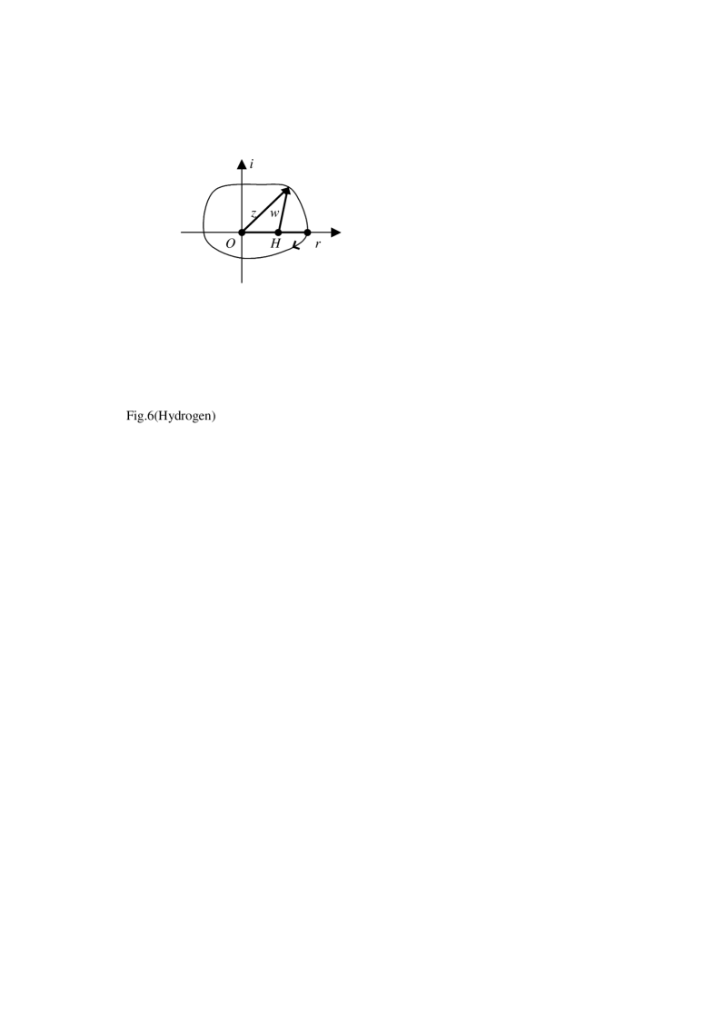
Figure 6: Unit circle contour for evaluating integral

$$\int\nolimits_{L} = \frac{1}{2}(\int\nolimits_{L}+\int\nolimits_{L-})=-\frac{1}{2}(\int\nolimits_{C_{\gamma}}+\int\nolimits_{C_{\delta}})$$ (58)

$$= \frac{\pi Ee^{2}}{\sqrt{m_{e}^{2}c^{4}-E^{2}}}-\pi\sqrt{j^{2}\hbar^{2}c^{2}-e^{4}}$$

Thus Eq.(14) becomes

$$\frac{1}{\hbar c}\int\nolimits_{0}^{\infty}\sqrt{(E+\frac{e^{2}}{r})^{2}-m_{e}^{2}c^{4}-\frac{j^{2}\hbar^{2}c^{2}}{r^{2}}}dr$$ (59)

$$= \frac{\pi E\alpha}{\sqrt{m_{e}^{2}c^{4}-E^{2}}}-\pi\sqrt{j^{2}-\alpha^{2}}$$

where $\alpha=e^{2}/\hbar c$ is known as the fine structure constant.

A.4 discussion: the motion over turning points

Following the sign change for imaginary momentum over turning points, discussed in the preceding section, we find that the periodic condition or standing wave condition in hydrogen atom may written as

$$2\int\nolimits_{a}^{b}\sqrt{\lambda-\frac{m^{2}}{\sin^{2}\theta}}d\theta=2\pi k$$ (60)

$$\frac{1}{\hbar c}\int\nolimits_{x}^{y}\sqrt{(E+\frac{e^{2}}{r})^{2}-m_{e}^{2}c^{4}-\frac{\lambda\hbar^{2}c^{2}}{r^{2}}}dr=\pi s$$ (61)

because the integrations in the regions over the turning points are eliminated automatically. What are their physical meanings ? A direct explanation is that it is not necessary for the electron to enter the regions over the turning points, in compliance with classical physics.

In addition, the residue theorem we used in the paper gives out accurate results for our integrations, not approximate ones.

References

- [1] E. G. Harris, Introduction to Modern Theoretical Physics, Vol.1&2, John Wiley & Sons, USA, 1975, p.263, Eq.(10-40).
- [2] See ref.[1], p.554, Eq.(20-9).
- [3] H. Y. Cui, LANL arXive.quant-ph/0102114, 2001.
- [4] H. Y. Cui, in the proceedings of annual meeting of Chinese Physical Socity, China Beijing, August, 2002.
- [5] J. E. Marsden, Basic Complex Analysis, W. F. Freeman and company, USA, 1973, p.229.
- [6] L. I. Schiff, Quantum Mechanics, third ed. McGrall-Hill, USA, 1968, p.486, Eq.(53.26).