Stable Spatial Langmuir Solitons.

Abstract

We study localized two- and three-dimensional Langmuir solitons in the framework of model based on generalized nonlinear Schrödinger equation that accounts for local and nonlocal contributions to electron-electron nonlinearity. General properties of solitons are investigated analytically and numerically. Evolution of three-dimensional localized wave packets has been simulated numerically. The additional nonlinearities are shown to be able to stabilize both azimuthally symmetric two-dimensional and spherically symmetric three-dimensional Langmuir solitons.

Starting from the early 70-th, the fundamental role of Langmuir solitons (LS) in strong plasma turbulence is commonly known Zakharov1972 ; Rudakov1974 . Formation of LS are connected with the plasma extrusion from the regions of strong high-frequency electric field and trapping of plasmons into the formed density well (caviton). However, in the previous simplified theoretical models, two-dimensional (2D) and 3D solitons occurs to be unstable with respect to a collapse: above some threshold power, the size of the structure shrinks infinitely, forming density singularity at finite time Zakharov1972 . Physically, when the size of collapson approaches few Debye radii $r_{D}$, it should damp rapidly which may result in fast plasma heating. Nevertheless, experimental observations AntipovNezlin1981 ; Tran82 ; Eggleston1982 ; Wong1984 ; Wong1985 of quasi-2D and 3D Langmuir collapse demonstrate saturation of wave-packet’s spatial scale at some minimum value being of order $(10\div 40)r_{D}$. It have been observed in Refs. Wong1984 ; Wong1985 that at times $t>50\omega_{Pi}^{-1}$, where $\omega_{Pi}$ is the ion plasma frequency, Langmuir wave packets show considerably slow dynamics (subsonic regime). To our best knowledge, these observations do not meet an appropriate theoretical explanation yet.

Various additional linear and nonlinear effects, such as higher-order dispersion Karpman96 ; Zakharov98 ; OurPRE03 , the saturation of nonlinearity ZakharovSobolevSynakh1971 ; VakhitovKolokolov ; OurPRE03 , nonlocal wave interaction DavydovaFischuk95 ; BangKrolikowskiWyllerRasmussen2002 ; Parola1998 ; KrolikovskiBangRasmussen2001 ; Brizhik2001 ; ZakrzewskiUFZ03 ; PerezGarciaKonotopPRE2000 , may arrest wave collapse both in 2D and in 3D Karpman96 ; VakhitovKolokolov ; Zakharov98 ; DavydovaFischuk95 ; BangKrolikowskiWyllerRasmussen2002 . As it is shown in Kuznetsov1976 , the local part of electron-electron nonlinearity (resulting from the interaction with the second harmonic) counteracts the contraction of wave packet. At the same time, the nonlocal contribution of the additional nonlinear term was omitted in Kuznetsov1976 , though it is of great importance for sufficiently narrow and intense wave packets. In this Letter we take into consideration both these extra nonlinear effects. As it will be shown below, the role of nonlocal nonlinearity is quantitatively even more significant. The nonlocal nonlinearity is of great importance not only when describing soliton formation in plasmas DavydovaFischuk95 ; PorkolabGoldman76 ; OurUFZh03 , but also in the theory of Bose-Einstein condensates or matter waves Parola1998 ; PerezGarciaKonotopPRE2000 ; KrolikovskiBangRasmussen2001 ; BangKrolikowskiWyllerRasmussen2002 , and in the construction of an adequate continuum model of the electron-phonon interaction in discrete 2D and 3D lattices Brizhik2001 ; ZakrzewskiUFZ03 .

The evolution of radial component of electric field strength $E$ of a Langmuir 2D and 3D wave packet is described by the set of equations:

$$\textrm{i}\frac{\partial E}{\partial t}+\frac{3}{2}\omega_{p}r_{D}^{2}\frac{\partial}{\partial r}r^{1-d}\frac{\partial}{\partial r}r^{d-1}E-\frac{\omega_{p}}{2}\frac{n_{1}}{n_{0}}E$$

$$-\frac{1}{48\pi mn_{0}\omega_{p}}\frac{E\left|E\right|^{2}}{r^{2}}+\frac{3}{2}\,\,\frac{E\Delta_{r}\left|E\right|^{2}}{48\pi mn_{0}\omega_{p}}=0,$$

$$\left(\frac{\partial^{2}}{\partial t^{2}}-c_{S}^{2}\Delta_{r}\right)\left(n_{1}+\frac{\Delta_{r}\left|E\right|^{2}}{16\pi m\omega_{p}^{2}}\right)=\frac{\Delta_{r}\left|E\right|^{2}}{16\pi M},$$

where azimuthal or spherical symmetry is supposed, $r$ – radial coordinate, $\Delta_{r}=\frac{\partial^{2}}{\partial r^{2}}+\frac{d-1}{r}\frac{\partial}{\partial r}$, $r_{D}$ – Debye radius, $\omega_{p}$ – electron plasma frequency, $d$ is the number of space dimensions, $m$ and $M$ are the electron and ion masses, $n_{0}$, $T_{e}$ – background electron density and temperature respectively and $c_{S}=\sqrt{T_{e}/M}$ is the ion sound speed, $n_{1}$ is the electron density perturbation. This equation set is valid if $W/nT<(kr_{D})^{-1}$, where $W=E^{2}/8\pi$, $k$ being the effective wave number of the packet. In Kuznetsov1976 , the similar set of equations for Langmuir wave field was derived, however, the nonlocal nonlinear terms were omitted.

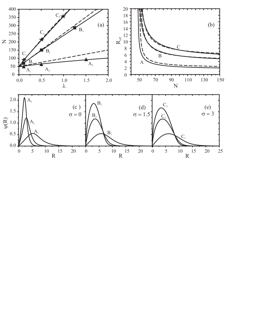
Figure 1: Two-dimensional Langmuir solitons: (a) EDD for $\sigma=0$ (A), $\sigma=1.5$ (B), and $\sigma=3.0$ (C); (b) Effective soliton width vs plasmon number; (c)-(e) soliton profiles for different $\sigma$. Each profile corresponds to the point marked at the EDD lines.

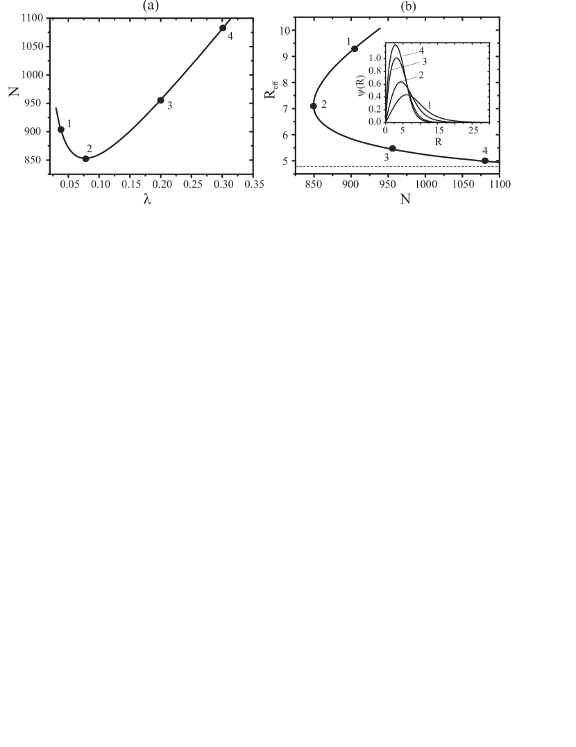
Figure 2: Three-dimensional Langmuir solitons. (a) Plasmon number $N$ vs nonlinear frequency shift $\lambda$ for $\sigma=1.5$; (b) Effective soliton width vs plasmon number. The inset: soliton profiles corresponding to the points marked at the $N(\lambda)$ and $R_{\textrm{eff}}(N)$ curves.

We consider subsonic motions and neglect the terms with time derivatives in the second equation of above set. As result, this set is reduced to the single partial differential equation:

$$\textrm{i}\frac{\partial E}{\partial t}+D\frac{\partial}{\partial r}\,r^{1-d}\frac{\partial}{\partial r}r^{d-1}E+BE\left|E\right|^{2}$$

$$+CE\Delta_{r}\left|E\right|^{2}-\Gamma\frac{E\left|E\right|^{2}}{r^{2}}=0,$$ (1)

where the coefficients $D$, $B$, $C$, $\Gamma$ are given by the expressions:

$$D=\frac{3}{2}\omega_{p}r_{D}^{2},\,\,\,B=\frac{\omega_{p}}{32\pi Mn_{0}c_{S}^{2}},$$

$$C=\frac{7}{96\pi mn_{0}\omega_{p}},\,\,\,\Gamma=\frac{1}{48\pi mn_{0}\omega_{p}}.$$

Equation (1) is closely related to nonlinear Schrödinger equation with modified linear term (proportional to $D$). The nonlinear part of this equation includes common cubic nonlinearity (term proportional to $B$) as well as nonlocal (term proportional to $C$) and local (term with $\Gamma$) parts of electron-electron nonlinearity.

Equation (1) conserves the following integrals: the plasmon number

$$N=\int\left|E\right|^{2}d\textbf{r},$$ (2)

and Hamiltonian:

$$H=D\int\left|r^{1-d}\frac{\partial}{\partial r}r^{d-1}E\right|^{2}d\textbf{r}-\frac{B}{2}\int|E|^{4}d\textbf{r}$$

$$+\frac{C}{2}\int\left(\nabla\left|E\right|^{2}\right)^{2}d\textbf{r}+\frac{\Gamma}{2}\int\frac{\left|E\right|^{4}}{r^{2}}d\textbf{r}.$$ (3)

Other integrals (momentum and angular momentum) are equal to zero in the case under consideration.

Let us show that the effective width $r_{\textrm{eff}}$

$$r_{\textrm{eff}}^{2}=\frac{1}{N}\int r^{2}|E|^{2}d\textbf{r},$$ (4)

of any wave packet governed by the Eq. (1) is bounded from below in the most interesting case of self-trapped wave packets having negative Hamiltonian. If both $C$ and $\Gamma$ in Eq. (1) are equal to zero, and $H<0$, collapse occurs. However, any of additional nonlinear terms (proportional to $C$ or $\Gamma$) prevents collapse in 2D as well as in 3D cases, or, in the other words, $r_{\textrm{eff}}$ is bounded from below.

Let us define

$$r_{1}^{2}=\frac{\int r^{2}\left|E\right|^{4}d\textbf{r}}{\int\left|E\right|^{4}d\textbf{r}},\,\,\,r_{2}^{2}=\frac{\int\left|E\right|^{4}d\textbf{r}}{\int\left|E\right|^{4}r^{-2}d\textbf{r}},$$

where all integrals are supposed to be finite. It is easy to show that

$$r_{1}^{2}>r_{2}^{2}.$$ (5)

Since Hamiltonian (3) is assumed to be negative, it is necessary that

$$B\int\left|E\right|^{4}d\textbf{r}>C\int\left(\nabla\left|E\right|^{2}\right)^{2}d\textbf{r}+\Gamma\int r^{-2}\left|E\right|^{4}d\textbf{r}.$$ (6)

Then we use the “uncertanity relation” of the form

$$r_{1}^{2}\int\left(\nabla\left|E\right|^{2}\right)^{2}d\textbf{r}>\alpha(d)\int\left|E\right|^{4}d\textbf{r},$$ (7)

where $\alpha=3/4$ in 3D case and $\alpha=1/2$ in 2D case. One can see from inequality (6) that $r_{2}^{2}>\Gamma/B$, thus, using Eq. (5) one gets $r_{1}^{2}>\Gamma/B$. Taking into account that for a localized wave packet $r_{\textrm{eff}}^{2}\geq r_{1}^{2}$, we finally obtain

$$r_{\textrm{eff}}^{2}>\textrm{max}\left\{\frac{\Gamma}{B},\,\,\frac{\alpha(d)}{2B}\left[C+\sqrt{C^{2}+\frac{4\Gamma C}{\alpha(d)}}\right]\right\}.$$ (8)

Thus, if $C\neq 0$ (or if $\Gamma\neq 0$), the wave packet can not be contracted to the size smaller than $\sqrt{C/B}$ (or $\sqrt{\Gamma/B}$).

By introducing the dimensionless variables:

$$R=\sqrt{\frac{3}{2}}\frac{r}{r_{D}},\tau=\frac{9}{4}\omega_{p}t,\Psi=E\sqrt{72\pi n_{0}T_{e}},$$

Eq. (1) is reduced to

$$\textrm{i}\frac{\partial\Psi}{\partial\tau}+\frac{\partial^{2}\Psi}{\partial R^{2}}+\frac{d-1}{R}\frac{\partial\Psi}{\partial R}-\frac{d-1}{R^{2}}\,\,\Psi+\Psi\left|\Psi\right|^{2}$$

$$+\sigma\Psi\Delta_{R}\left|\Psi\right|^{2}-\frac{\Psi\left|\Psi\right|^{2}}{R^{2}}=0,$$ (9)

where $\sigma=7/2$. (In the limit $\sigma=0$ equation (9) reduces to equation (18) of Ref. Kuznetsov1976 .) We will keep $\sigma$ as free parameter to study the impact of nonlocality on the properties of 2D and 3D Langmuir solitons and bearing in mind the other possible applications of model equation (9).

Soliton solutions of Eq. (9) have a form $\Psi(R,\tau)=\psi(R)\exp{\textrm{(}{i}\lambda\tau)}$, where $\lambda$ is the nonlinear frequency shift of the soliton. The radial soliton profiles $\psi(R)$ are found from the equation

$$-\lambda\psi+\frac{\partial^{2}\psi}{\partial R^{2}}+\frac{d-1}{R}\frac{\partial\psi}{\partial R}-\frac{d-1}{R^{2}}\,\,\psi+\psi\left|\psi\right|^{2}$$

$$+\sigma\psi\Delta_{R}\left|\psi\right|^{2}-\frac{\psi\left|\psi\right|^{2}}{R^{2}}=0.$$ (10)

We will start our consideration with 2D Langmuir solitons. Note the formal analogy between Eq. (10) for radial electric field component in 2D case and NLSE for vortex solitons $\psi(R)\exp{(\textrm{i}m\varphi)}$ with topological charge $m=1$ (see, e.g. OurPRE03 ). However, in spite of zero value of wave intensity at the soliton center, it has no phase dislocation and corresponds to the ground state with minimum energy and zero angular momentum. In the considered case of Langmuir wave structures, the phase does not depend on the radial coordinate, thus in Eq. (10) $\psi(R)$ may be considered as real function.

Stationary states of Eq. (1) were investigated analytically and numerically. Analytical approach employs approximate variational method (see, e.g. Anderson1983 ) with the normalized trial function of the form

$$E(r)=\sqrt{N\mu^{2}/\pi}\,\,\xi\exp{(-\xi^{2}/2)},\,\,\,\xi=\mu r,$$ (11)

where the variational parameter $\mu$ characterizes the inverse soliton’s width: $\mu=1/(\sqrt{2}\,r_{\textrm{eff}})$. We have returned to the nonscaled variables for variational analysis. The trial function (11) has a correct asymptotic near the soliton center. The Gaussian profile gives a good approximation to soliton solutions, since, as it was argued in BangKrolikowskiWyllerRasmussen2002 it represents an exact solution in the limit case of strong nonlocality. The variational parameter $\mu_{0}$ corresponding to stationary solutions of the form (11), is readily found after standard procedure Anderson1983 :

$$\mu_{0}^{2}=\mu_{*}^{2}\,(N-N_{0})/N,$$ (12)

where $\mu_{*}^{2}=B/(4C+2\Gamma)$, $N_{0}=16\pi D/B$. Thus, 2D Langmuir solitons are formed only when some threshold value of plasmon number is exceeded (i.e. if $N>N_{0}$). One can see that $\mu_{0}\to\mu_{*}$ at $N\gg N_{0}$, so that the effective width is bounded from below: $r_{\textrm{eff}}\geq\sqrt{(2C+\Gamma)/B}$, which agrees with previous general estimate given by Eq. (8).

The boundary-value problem described by the Eq. (10) with zero boundary conditions at the soliton’s center ($R=0$) and at infinity ($R\to\infty$) was solved numerically by the shooting method. Solitons form two-parameter family with parameters $\sigma$ and $\lambda$. For each given nonlocality parameter $\sigma$ we present the dependence $N(\lambda)$ known as “energy dispersion diagram” (EDD), which are given in Fig. 1 (a). Note that all solitons are stable, which is similar to Vakhitov-Kolokolov criterion VakhitovKolokolov , since $\partial N/\partial\lambda>0$. To excite stable two-dimensional Langmuir soliton, the threshold value $N_{0}$ of input power (critical plasmon number) should be exceeded. Variational approach predicts normalized critical plasmon number to be $N_{0}=16\pi$. This is in a very good agreement with our numerical results, where $N_{0}\approx 48.3$. Moreover, this simple variational analysis gives a good description for all EDDs, and variational dependence $N(\lambda)$ fits better the computed one when the parameter $\sigma$ grows. It is illustrated in the Fig. 1 (a) for different $\sigma$. One can see that at $\sigma=0$, the shape of soliton differs sufficiently from the simple profile of the form (11) [compare Fig. 1 (c) with Fig. 1 (d),(e)]. The typical soliton profiles are plotted in Fig. 1 (c)-(e). At the same plasmon number, the soliton width is larger for solutions of Eq. (10) with nonlocal nonlinearity ($\sigma>0$) than for solutions with $\sigma=0$.

As it was stressed above, the effective width of Langmuir wave packet in our model is bounded from below. Figure 1 (b) represents the effective soliton width as function of plasmon number. The $R_{\textrm{eff}}$ decays monotonically and saturates at some nonzero minimum value $R_{\textrm{min}}$. This minimum width increases when parameter $\sigma$ increases, as it was estimated above [see Eq. (8)]. In the dimensional variables, the minimum diameters of 2D Langmuir structures are of order $10r_{D}$ which is in a good agreement with those observed experimentally in Eggleston1982 .

We have performed similar analytical and numerical study for 3D radially-symmetric solitons. The corresponding $N(\lambda)$ and $R_{\textrm{eff}}(N)$ dependencies are shown in Fig. 2 (a), (b). In the 3D case, plasmon number depends on nonlinear frequency shift $\lambda$ non-monotonically, and the only stable soliton branch corresponds to $\partial N/\partial\lambda>0$, as it follows from Vakhitov-Kolokolov criterion. Therefore, in the 3D case, the threshold plasmon number $N_{cr}$ needed to excite stable Langmuir soliton should be obtained from condition $\partial N/\partial\lambda=0$. Similarly to the 2D case, the effective width $R_{\textrm{eff}}$ of stable solitons decays monotonically when plasmon number $N$ grows, and $R_{\textrm{eff}}\to R_{\textrm{min}}$ at $N\gg N_{cr}$. We have found the threshold value to be of order $N_{cr}\approx 850$.

We have investigated evolution of radially symmetric Langmuir structures numerically in the framework of Eq. (9). The integration time step was splitted into the linear and nonlinear parts, and both of them were performed in the radial coordinate domain. During the simulations, the conservation of integrals (2) and (3) has been verified, and if the change of any integral exceeded 1%, the modelling was stopped. We used two types of initial conditions: (i) perturbed stationary soliton solution of Eq. (10) which was found numerically, and (ii) the Gaussian-like profile. At the boundaries we assumed that $\partial\left[\Psi(R,t)/R\right]/\partial R=0$ at $R\to 0$ and $\Psi(R,t)=0$ at $R\to\infty$.

Stability properties of Langmuir solitons were found to be in a very good agreement with our analytical predictions. Any localized wave packet having the number of quanta below the threshold value $N<N_{cr}$ always spreads out, while an initially more intense packet with $N>N_{cr}$ may form a localized structure after irradiating a portion of plasmons. The dynamics of intense wave packet with $N>N_{cr}$ is very intriguing. Figure 3 represents the different evolution scenarios of perturbed 3D Langmuir solitons. The amplitude and effective width of slightly perturbed soliton solution belonging to the stable branch (with $\partial N/\partial\lambda>0$) oscillate in time as it is seen in Fig. 3 (a). However, when perturbed, an unstable stationary solution (having $\partial N/\partial\lambda<0$) manifests different evolution pattern: it can either monotonically spread out [see Fig. 3 (c)] or develop quasiperiodical motion [see Fig. 3 (b)], depending on the initial perturbation. The latter quasiperiodical behavior resembles the oscillations between two opposite extreme states discussed in BangKrolikowskiWyllerRasmussen2002 ; PerezGarciaKonotopPRE2000 . The initial increase of wave packet’s intensity is followed by quasiperiodical oscillations with rather large amplitude. Thus, the additional nonlinearities actually prevent catastrophic collapse of any 3D Langmuir wave packets. The similar regime is known as ”frustrated collapse” PerezGarciaKonotopPRE2000 in theory of Bose-Einstein condensates with nonlocal nonlinear interaction.

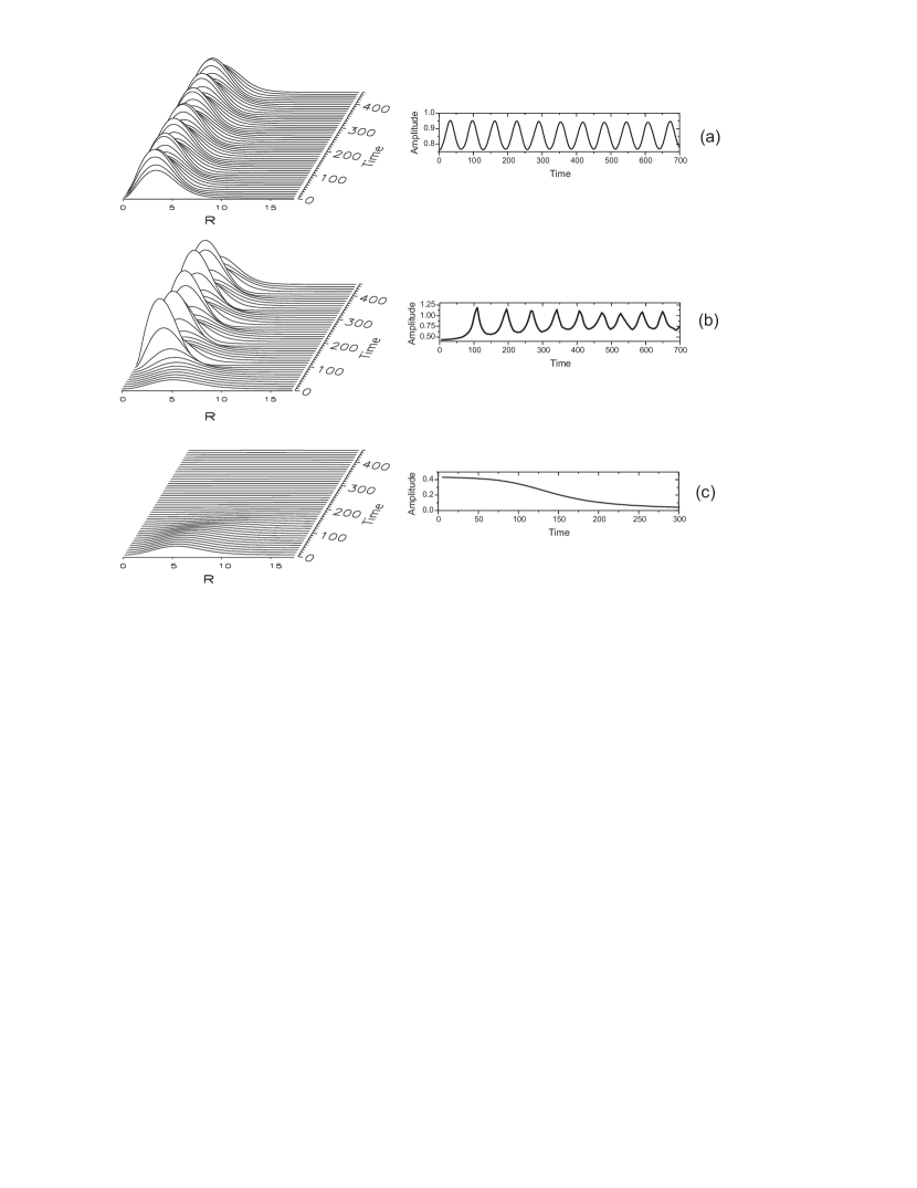
Figure 3: Typical examples of evolution of 3D Langmuir wave packets ($\sigma=1.5$). Left panels represent distributions of wave intensity $|\Psi(R,t)|^{2}$. Right panels show wave packet’s amplitude $\Psi_{\textrm{max}}$ vs time. (a) perturbed stable soliton with $\lambda=0.1$; perturbed soliton from unstable branch at $\lambda=0.03$ and different perturbations: (b) demonstrates quasiperiodical dynamics; (c) spreads out.

Our considerations are in a qualitative agreement with experimental observations of Langmuir wave structures in unmagnetized laboratory plasmas Wong1984 ; Wong1985 . On the slow (subsonic) stage of evolution, which was observed at time $t>50\omega_{Pi}^{-1}$, the field envelope almost stopped its radial contraction and the size remained approximately unchanged ($r$ is of order of few tens of $r_{D}$). It is important to note that according to Wong1984 ; Wong1985 at this stage of Langmuir structure evolution, the beam-wave resonance is detuned and the beam decouples from the wave. Nevertheless, the common Zakharov set of equations describes field evolution only for rather short time ($t<50\omega_{Pi}^{-1}$) and then its prediction drastically deviates from experimental facts because the wave packet becomes too intense (at peak $E_{max}^{2}/4\pi nT\sim 1$) and too narrow. As it was demonstrated above, the electron-electron nonlinearity plays a crucial role in Langmuir structure behavior and it gives the qualitative explanation of saturation of the wave packet contraction. The dissipative effects such as Landau and transit-time damping seems to be negligible for structures of several tens Debye’s radius characteristic size. Certainly, the wave packet may interact with high-energy electrons, therefore, after a long time (of order of several hundreds of $\omega_{Pi}^{-1}$), it may eventually damp due to wave absorption. Our considerations are valid at stage when nonlocal nonlinearities come into play and considerably slow down the wave packet contraction but the wave absorption is still not essential.

In conclusion, we have performed analytical and numerical studies of spatial (2D and 3D) Langmuir solitons in the framework of model based on generalized nonlinear Schödinger equation including both local and nonlocal electron-electron nonlinearities. Their influence on intense and narrow Langmuir wave packets are of the same order, and both nonlinearities should be taken into account simultaneously. Any of them is able to arrest the Langmuir collapse. Both nonlinearities lead to the saturation of soliton width with an increase of the energy, but quantitatively the effect of nonlocal nonlinearity is more significant. All 2D Langmuir solitary structures are stable, while in 3D case, two soliton branches coexist, one is stable and the other is unstable. When perturbed, stable solitons demonstrate centrosymmetric oscillations. As for 3D solitons from the unstable branch, they may either spread out or oscillate quasiperiodically depending on perturbation applied.

References

- (1) V.E. Zakharov. Sov.Phys.JETP, 35:908–914, 1972.
- (2) L. I. Rudakov. ZhETP Letters, 19:729–733, 1974.
- (3) S. V. Antipov, M. V. Nezlin, A. S. Trubnikov, and I. V. Kurchatov. Physica D Nonlinear Phenomena, 3:311–328, 1981.
- (4) P. Leung, M. Q. Tran, and A. Y. Wong. Plasma Physics, 24:567–575, 1982.
- (5) D. L. Eggleston, A. Y. Wong, and C. B. Darrow. Physics of Fluids, 25:257–261, 1982.
- (6) A. Y. Wong and P. Y. Cheung. Physical Review Letters, 52:1222–1225, 1984.
- (7) P. Y. Cheung and A. Y. Wong. Physics of Fluids, 28:1538–1548, 1985.
- (8) V.I. Karpman. Phys. Rev. E, 53:1336–1339, 1996.
- (9) V. E. Zakharov and E. A. Kuznetsov. Journal of Experimental and Theoretical Physics, 86:1035–1046, 1998.
- (10) A.I. Davydova, T.A. Yakimenko and Yu.A. Zaliznyak. Phys. Rev. E, 67:026402, 2003.
- (11) V.V. Zakharov, V.E. Sobolev and V.C. Synakh. Sov. Phys. JETP, 33:77, 1971.
- (12) A.A. Vakhitov, N.G. Kolokolov. Izv. VUZov: Radiofizika, 16:1020–1028, 1973.
- (13) T.A. Davydova and A.I. Fischuk. Ukrainian Journal of Physics, 40:487–494, 1995.
- (14) O. Bang, W. Krolikowski, J. Wyller, and J. J. Rasmussen. Physical Review E, 66:046619, 2002.
- (15) A. Parola, L. Salasnich, and L. Reatto. Phys.Rev. A, 57:3180–3183, 1998.
- (16) J.J. Krolikovski, W. Bang O. Rasmussen and J. Wyller. Phys. Rev. E, 64:016612, 2001.
- (17) L. Brizhik, A. Eremko, B. Piette, and W. J. Zakrzewski. Physica D Nonlinear Phenomena, 159:71–90, 2001.
- (18) W. J. Zakrzewski. Ukrainian Journal of Physics, 48(7):630–637, 2003.
- (19) V. M. Pérez-García, V. V. Konotop, and J. J. García-Ripoll. Phys.Rev.E, 62:4300–4308, 2000.
- (20) E.A. Kuznetsov. Soviet Journal of Plasma Physics, 2(2):187–181, 1976.
- (21) M. Porkolab and M.V. Goldman. Phys. Fluids, 19:872–881, 1976.
- (22) T.A. Davydova and A.I. Yakimenko. Ukrainian Journal of Physics, 18:623–629, 2003.
- (23) D. Anderson. Phys. Rev. A, 27(6):3135–3145, 1983.